Download
1 / 34
340 likes | 533 Vues
Estimating biophysical parameters from CO 2 flask and flux observations. Kevin Schaefer 1 , P. Tans 1 , A. S. Denning 2 , J. Collatz 3 , L. Prihodko 2 , I. Baker 2 , W. Peters 1 , A. Andrews 1 , and L. Bruhwiler 1.

E N D
Estimating biophysical parameters from CO2 flask and flux observations Kevin Schaefer1, P. Tans1, A. S. Denning2, J. Collatz3, L. Prihodko2, I. Baker2, W. Peters1, A. Andrews1, and L. Bruhwiler1 1NOAA Climate Monitoring and Diagnostics Laboratory, Boulder, Colorado2Dept. of Atmospheric Science, Colorado State University, Fort Collins, Colorado3Goddard Space Flight Center, Greenbelt, Maryland
Objective • Understand processes driving terrestrial CO2 fluxes • Technique: estimate model parameters using data assimilation • Model: • Simple Biosphere (SiB) • Carnegie-Ames-Stanford Approach (CASA) • Observations: • CO2 concentrations from CMDL flask network • CO2 concentrations & fluxes from towers
Status • 2-year NAS Postdoc fellowship @ CMDL • Joint effort: CMDL & CSU • SibCasa in final testing • Switching to EnKF • Preliminary results • Offline with SiB2 & TransCom fluxes • Single point @ WLEF
Combined SibCasa Model • Simple Biosphere (SiB) • Biophysical • Good photosynthesis model • High time resolution • CASA • Biogeochemical • Good respiration model • Coarse time resolution • SibCasa • Good GPP Model • Good respiration model • High time resolution
Which parameters to estimate? High no excuse no way Influence no problem no bother Low Low High Uncertainty
Hourly and monthly average net CO2 fluxes WLEF WLEF Tall Tower in Wisconsin
SibCasa Observed Monthly Observed vs. SibCasa Fluxes at WLEF Net CO2 Flux (mmole/m2/s) Date (year)
SibCasa Observed Hourly Observed vs. SibCasa Fluxes at WLEF Net CO2 Flux (mmole/m2/s) Date (year)
SibCasa Observed SibCasa diurnal cycle too small at WLEF June 2-5, 1997 Net CO2 Flux (mmole/m2/s) Date (year)
Sample Estimate: Respiration Temperature Response (Q10) Q10 = 3.0 Q10 = 2.0 Scaling Factor (-) Q10 = 1.0 Soil Temperature (K)
Data Assimilation: Minimize Cost function (F) • Optimize using Marquardt-Levenberg method (variant of inverse Hessian) • No model adjoint: approximate F slope
Q10 Cost Function at WLEF (no a priori) • Hourly Obs: aliasing Q10 to “fix” diurnal cycle
Initial Slow Pool Cost Function at WLEF • Monthly Obs: aliasing Slow to “fix” low GPP in 1998 Equilibrium Pool Size
Conclusions • We can estimate model parameters from CO2 data • Be careful about data assimilation “correcting” for model flaws
What process information can we extract from CO2 flask and flux tower observations? Atmospheric Transport Net Flux Flux Tower Fossil Fuel Flask Net Flux Ocean Processes Biosphere Processes
Objectives • Use model physics to better understand mechanisms that drive CO2 fluxes • Optimize model parameters to best match model output & observations • Estimate hard-to-measure parameters: Q10, turnover, pool sizes, etc. • Joint effort: CMDL & CSU
Postdoc Plan • 6 Months for Software development • Add geochemistry from CASA to SiB2 • 8 months for simulations and testing • Flux towers first, then flasks • 6 months writing papers • Status: 3 months into SiB-CASA development
DAS Setup • Combine SiB3 with CASA • SiB3: Photosynthesis & turbulent fluxes • CASA: biogeochemistry and respiration • Integrate Sibcasa into TM5 • Use Ensemble Kalman Filter (EnKF)
DAS Experiments • Single point: Sibcasa & flux tower data • Offline: Sibcasa & Transcom3 fluxes • Compare NCEP, ECMWF, GEOS4 reanalysis • Integrated: Sibcasa in TM5 & flask data
Problems • Parameter Estimation • Parameter compensation • Model/data biases • EnKF • 3-D [CO2] field from sparse flask observations • How to incorporate CO2 memory • How to go from parameter to flask • Number ensemble members
Data Assimilation: Minimize Cost Function (F) y = observations f(x) = model output E = uncertainty x = parameter to estimate
Data Assimilation: Minimize Cost function (F) • Variance between modeled & observed fluxes observed flux SiB2 flux parameter a priori a priori uncertainty flux uncertainty
Data Assimilation: Minimize Cost function (F) • Iterate using Marquardt-Levenberg method (variant of inverse Hessian) • Approximate Jacobian:
CO2 Flask Measurements Transport Models SiB2 TransCom Inversion Assimilation T Q10 Estimated NEE Modeled NEE LAI Weather Data Assimilation: Minimize Cost function (F) Iterate
Ensemble Kalman Filter (EnKF) • Use ensemble statistics to approximate terms in Kalman gain equation • Run ensemble ~100 members • No adjoint required • Experimental: still under development
History of Kevin • 1984: BS in Aerospace Engineering • 1984-1993: NASA • Space Shuttle, Space Station • Mission to Planet Earth • 1994-1997: White House • 1997-2004: CSU Atmospheric Science
Kevin’s Family Susy Jason
CO2 Ta Rha T6 W1 T5 T4 W2 T3 T2 W3 T1 Simple Biosphere Model, Version 2 (SiB2) NEE=R-GPP SH LH Tc Canopy Canopy Air Space GPP R Snow Tg Soil 11 to 45-year simulations 10-min time step
SiB2 Input • National Centers for Environmental Prediction (NCEP) reanalysis • 1958-2002, every 6 hours, 2x2º resolution • European Centre for Medium-range Weather Forecasts (ECMWF) reanalysis • 1978-1993, every 6 hours, 1x1º resolution • Leaf Area Index: Fourier-Adjustment, Solar zenith angle corrected, Interpolated Reconstructed (FASIR) Normalized Difference Vegetation Index (NDVI) data • 1982-1998, monthly, variable resolution
NOAA’s global flask network • Run transport backwards to estimate CO2 fluxes • Compare estimated & SiB2 regional fluxes
Initial Coarse Woody Debris Pool at WLEF • Monthly Obs: aliasing to fix low GPP in 1998 • Hourly Obs: aliasing to “fix” diurnal cycle Equilibrium Pool Size
Q10 Estimated from Transcom Fluxes Biome Q10 (-) Tropical broadleaf evergreen forest Broadleaf deciduous forest Broadleaf-needleleaf forest Needleleaf forest Needleleaf-deciduous forest Tropical Grasslands Semi-arid grasslands Broadleaf shrubs with bare soil Tundra Desert Agriculture and C3 grasslands 1.2 ± 0.1 2.2 ± 0.3 1.9 ± 0.1 2.6 ± 0.1 2.2 ± 0.1 1.4 ± 0.0 1.6 ± 0.1 1.7 ± 0.2 2.1 ± 0.2 2.6 ± 0.3 1.6 ± 0.0
Flasks: Turnover (T) and Q10 Biome T (mon) Q10 (-) Tropical broadleaf evergreen forest Broadleaf deciduous forest Broadleaf-needleleaf forest Needleleaf forest Needleleaf-deciduous forest Tropical Grasslands Semi-arid grasslands Broadleaf shrubs with bare soil Tundra Desert Agriculture and C3 grasslands 12.8 ± 0.81.2 ± 0.1 13.3 ± 2.22.2 ± 0.3 13.6 ± 0.81.9 ± 0.1 12.9 ± 0.52.6 ± 0.1 12.8 ± 0.42.2 ± 0.1 12.8 ± 0.41.4 ± 0.0 12.4 ± 1.01.6 ± 0.1 16.3 ± 1.91.7 ± 0.2 12.4 ± 1.02.1 ± 0.2 12.9 ± 2.42.6 ± 0.3 12.8 ± 0.41.6 ± 0.0
Global Estimated T and Q10 • Global Q10 = 1.67±0.04 • Agrees well with published values (1.6-2.4) • Q10 increases with shorter time scales • Global T = 12.7 ±0.8 months • Represents only fast turnover pools • Average between autotrophic & heterotrophic • Need more carbon pools in SiB2