Download

1 / 75
750 likes | 928 Vues
Applications of non-equilibrium statistical mechanics . Differences and similarities with equilibrium theories and applications to problems in several areas. Birger Bergersen Dept. Of Physics and Astronomy University of British Columbia birger@phas.ubc.ca. Overview.

E N D
Applications of non-equilibrium statistical mechanics Differences and similarities with equilibrium theories and applications to problems in several areas. Birger Bergersen Dept. Of Physics and Astronomy University of British Columbia birger@phas.ubc.ca
Overview • Overview of equilibrium systems: Ensembles, fluctuations , detailed balance, equations of state, phase transitions, broken symmetry, information theory. • Steady states vs. Equilibrium: Linear response, Onsager coefficients, variational principles, equilibrium “economics”, approach to equilibrium, Le Chatelier’s principle. • Oscillatory reactions: Belousov –Zhabotinsky reaction, brusselerator. • Effects of delay: Logistic equation with delayed carrying capacity • Inertia: Transition to turbulence • Bachelier-Wiener processes, Master equation, Birth and death, Fokker Planck equation, Brownian motion, escape probability, stochastic resonance, Brownian motors, Parrondo games. • Other processes: Material failure, multiplicative noise, income distribution, Pareto tail. • Levy distributions, colored noise,
Equilibrium: ensembles Insulating walls • Microcanonical ensemble: • Canonical ensemble: N,E,V specified Entropy S maximum subject to constraints Temperature T, pressure P, chemical potential μ fluctuating Heat bath at temperature T Helmholtz free energy A=E-TS minimum subject to constraints. Competition between energy and entropy. Entropy S , energy E, pressure, chemical potential fluctuating T,V,N specified
P • Gibbs ensemble G=E-TS+PV =μN minimum Gibbs-Duhem relation E=TS+ μN-PV valid if E,N,V,S extensive μ,T,P intensive Extensive= proportional to system size Intensive= independent of system size • Grand canonical ensemble Heat bath P,T,N specified Porous walls N,P,S fluctuating Grand potential Ω=-PV minimum Heat bath μ, V, T specified
Canonical ensemble dA =-SdT -PdV +μdN Example isothermal athmosphere If atmospheric pressure at height h=0 is p(0) and m the mass of a gas molecule
Canonical fluctuations • ...
I assume that what we done so far are things you have seen before, but to refresh your memory let us do some simple problems: Problem 1: In the micro-canonical ensemble the change in energy E, when there is an infinitesimal change in the control parameters S,V, N is dE= TdS-PdV+μdN So that T=∂E/ ∂S, P=- ∂E/ ∂V, μ= ∂E/ ∂N a. Show that if two systems are put in contact by a conducting wall their temperatures a equilibrium will be equal. b. Show that, if the two systems are separated by a frictionless piston, their pressures will be equal at equilibrium. c. Show that if they are separated by a porous wall the chemical potential will be equal on the two sides at equilibrium.
Solution: Instead of considering the state variable E as E(S,V,N) we can treat the entropy as S(E,V,N) dS=E/T dE +P/T dV –μ/ T dN Or 1/T=∂S/ ∂E Let E=E₁+E₂ be the energy of the compound system and the entropy is S=S ₁+S₂. At equilibrium the entropy is maximum or Since ∂E₁ / ∂E₂=-1 we find 1/T₁ =1/T₂ or T₁ =T₂ . Similar arguments for the case of the piston tells us that at equilibrium P₁/T₁ = P₂/T₂. But, since T₁ =T₂, P₁= P₂. The same argument tells us that μ₁= μ₂. Note that if the two systems are kept at different temperatures, the entropy is not maximum, when the pressure is equal as required by mechanical equilibrium! ∂
Problem 2: If q and p are canonical coordinated and momenta the number of quantum states between q and q+dq, p and p+dp are dp/dq/h, where h is Planck’s constant. If a particle om mass m is in a 3D box of volume V its canonical partition function is The partition function for an ideal gas of N identical particles is The factor N! comes about because we cannot tell which particle is in which state. Find expressions for the Helmholz energy A, the mean entropy S and the mean energy E and the pressure P Two ideal gases with N₁=N₂=N molecules occupy separate volumes V₁=V₂=V at the same temperature. They are then mixed in a volume 2V. Find the entropy of mixing. Show that there is no entropy change if the molecules are the same!
Solution: We have For large N we can use Stirlings formula ln N!=N ln N-N and find The entropy can be obtained from S=-∂A/ ∂T, and Similarly E=A+TS=3nkT/2 and P=-∂A/ ∂V=NkT If the two gases are different the change in entropy comes about because V→2V for both gases. Hence, ∆S=2Nk ln 2 If the two gases are the same there is no change in the total entropy.
Problem 3. Maxwell speed distribution Assuming that the number of states with velocity components between is proportional to and that the energy of a molecule with speed is find the probability distribution for the speed. Find the average speed The mean kinetic energy The most probable speed i.e. the speed for which
Solution: Going to polar coordinate we find that To find the proportionality constant we use after some algebra: Integrating we find
Principle of detailed balance The canonical ensemble is based on the assumption that the accessible states j have a stationary probability distribution π(j)=exp(-βE(j))/Z(β) This distribution is maintained in a fluctuating environment in which the system undergoes a series of small changes with probabilities P(m←j). For the distribution to be stationary it must not change by transitions in and out of state π(m)=∑ P(j←m) π(m)= ∑ P(m←j) π(j) This is satisfied by requiring detailed balance: P(j ←m)/P(m ←j)= π(j)/ π(m)=exp(-β(E(j)-E(m)) In a equilibrium simulation we get the correct equilibrium properties, by satisfying detailed balance and making sure there is a path between all allowed states. We can ignore the actual dynamics (Monte Carlo method). Very convenient! j j
Equations of state The equilibrium state of ordinary matter can be specified by a small number of control variables. For a one component system the Helmholtz free energy is A=A(N,V,T). Other variables such as the pressure P, the chemical potential μ, the entropy S are given by equations of state μ=∂A/ ∂N, P= - ∂A/ ∂V, S=- ∂A/ ∂T An approximate equation of state describing non-ideal gases Is the van der Waals equation which obtains from the free energy Comparing with the monatomic ideal gas expression We interpret the constant a as a measure of the attraction between molecules outside a hard core volume b
Equilibrium phase transitions For special values of the control parameters (P,N,T in the Gibbs ensemble) the orderParameters (V,μ,S) changes abruptly. P and T for a single component system when solids/liquid and gas/liquid coexists at equilibrium is shown at the top while the specific volume v=V/N for a given P is below. The gas/liquid and solid/liquid transition are 1st order (or dis- continuous). The critical endpoint of the latter is a 2nd order (or continuous ). Specific heat and fluctuations diverge at critical point.
Problem 4: Van der Waals equation. Express the equation as a cubic equation in v=V/N. Find the values for which the roots coincide. Rewrite the equation in terms of the reduced variables. the resulting equation is called the law of corresponding states. d. Discuss the behaviour of the isotherms of the the law of corresponding states.
Solution: Multiplying out and dividing by a common factor we find When the roots are equal this expression must be on the form comparing term by term we find after some algebra Again, after some algebra we find in terms of the new variables the law of corresponding states We next plot p(v,t) for different values of t
For t<1 there is a range of pressures p₁<p<p₂ with 3 solutions . The points p₁ and p₂ are spinodals. In the region between them the compressibility -∂P/∂V is negative and the system is unstable. The equilibrium state has the lowest chemical potential μ ←t=1.1 P t=1 → ←t=0.9 We have μ=(A+PV)/N so that dμ=(SdT+VdP)/N μ₂- μ₁=∫²₁=∫VdP/N The equilibrium vapor pressure is when the areas between the horizontal line and the isotherms are equal. Between the equilibrium pressure and the spinodal there is a metastable region. Dust can nucleate rain drops. If particles too small surface tension prevents nucleation. VdW theory gualitatively but not quantitatively ok.
Symmetry breaking: Alben model. A large class of equilibrium systems characterized by a high temperature symmetric phase and low temperature broken symmetry phase. Some examples: Magnetic models: Selection of spin orientation of “spins”, Ising model, Heisenberg model, Potts model.... Miscibility models: High temperature solution phase separates at lower temperatures Many other models in cosmology, particle and condensed with analogies in other fields. The Alben model is a simple mechanical example. An airtight piston of mass M separates two regions, each containing N ideal gas molecules at temperatureT. The piston is in a semicircular tube of cross section a. The “order parameter” of the problem is the angle Φ of the piston.
The free energy of an ideal gas is A=-NkTln (V/N)+terms independent of V, N yielding the equation of state PV=-∂A/ ∂V=NkT We add the gravitational potential energy to obtain A=M gRcosφ- NkT(ln [aR(π/2+ φ)/N]+ln [aR(π/2+-φ)/N] Minimizing with respect to φ gives 0= ∂A/ ∂ φ=-MgR sin φ-8NkT φ/(π²-4 φ²) This equation has a nonzero solution corresponding to minimum for T<T₀=MgR π²/(8Nk) The resulting temperature dependence of the order parameter is shown below to the left. To the right we show the behavior if the amount of gas on the two sides is N(1±0.05)
At equilibrium: • Second law: Variational principles apply: entropy maximum subject to constraints → free energy minimum . System stable with reversible, Gaussian fluctuations (except at phase transitions, continuous or discontinuous) → No arrow of time, detailed balance. • Zeroth law: Pressure, temperature chemical potential constant throughout system. • No currents (of heat, charge, particles) • Thermodynamic variables: Extensive (proportional to system size, N,V,E,S), or intensive (independent of size, μ,T,P). Law of existence of matter. • Typical fluctuations proportional to square root of size
Steady state vs. equilibrium: • Steady states are time independent, but not in equilibrium. Heat current Electric current T T+Δ J Q No zeroth law! Gradients of temperature, chemical potential and pressure allowed. Osmosis Salt water Fresh water
Energy Raw materials Labour Capital Economy Economy Waste Products Wages Profits If no throughput there is no economy! Economic “equilibrium” an oxymoron.
Equilibrium “economics” • N = # of citizen >>1w = W/N= average incomeMost probable income distributionp(w)=exp(-x/w)/wAverage income analogous to thermodynamic temperature.Problem: Income inequality varies from society to society! More parameters needed!
In non-equilibrium steady state entropy not maximized (subject to constraint). Example: Two gas containers of equal size are connected by A capillary. One is kept at a higher temperature than the other by contact with heat baths. If the capillary is not too thin (compared to mean free path of molecules ) system will reach mechanical equilibrium with constant pressure. The cold container will then have more molecules than the hot one. P, V Tc P, V Th The entropy per molecule is higher in hot gas. If entropy maximum subject to temperature constraint molecules would move from cold to hot. This does not happen! Chemical potential will be different on the two sides in steady state. Steady states not governed by variational principle! Zeroth law does not apply!
Systems near equilibrium • Ohm’s law: Electrical currentV=R IV=voltage, R= resistance, I=current • Fick’s law of diffusion • Stokes law for settling velocity Many similar laws!
More subtle effects: Temperature gradient in bimetallic strip produces electromotive force → Seebeck effect Electric current through bimetallic strip leads to heating at one end And cooling at the other → Peltier effect Dust particle moves away from hot surface towards cooler region. →Thermophoresis. Particles in mixture may selectively move Towards hotter or cooler regions → Ludwig-Soret effect In rarefied gases a temperature gradient may a pressure gradient → thermomolecular effect Economic analogies? Wealth gradient may cause migration, emigration and ghetto formation.
Le Chatelier’s principle Any change in concentrations, volume or pressure is counteracted by shift in equilibrium that opposes change. If a system is disturbed from equilibrium , it will return monotonically towards equilibrium as disturbance is removed (no overshoot). In neoclassical economics it has been suggested that if supply exceeds demand, prices will fall, production cut and equilibrium restored. A similar process should occur if demand exceeds supply But is this true?
Belousov-Zhabotinsky reaction In the 1950s Boris Pavlovich Belousov discovered an oscillatory chemical reaction in which Cerium IV ions in solution is reduced by one chemical to Ce III and subsequently oxidized to Ce IV causing a periodic color change. Belousov was unable to publish his results, but years later Anatol Zhabotinsky repeated the experiments and produced a theory . By now many other chemical oscillators have been found.
A linear stability analysis of the fixed point in parameter space is shown in the picture to the right. Trajectories of the concentrations X and Y are shown below. ↘ ↘ ↘ ↘ Le Chatelier’s principle does not apply because the system is driven, A,B must be kept constant. Reactions are irreversible.
Problem 5: LotkaVolterra model Big fish eat little fishes to survive. The little fish reproduce at a certain net rate, and die by predation. The rate model rate eqs are Simplify the model by introducing new variables b. Find the steady states of the populations and their stability. Discuss the solutions to the rate equations. c. In the model, the populations of little fish grows without limits if the big fish disappear. Modify the little fish equation to add a logistic term, with K the carrying capacity How does this change things? d. If the population of big fish becomes too small it may become extinct. Modify model to include small immigration rates. Neglect the effect of finite carrying capacity.
Solution: a. With the substitutions the equations become dy/dτ=-ry(1-x); dx/dτ=x(1-y) b. There are two steady states {x=0,y=0}, and {x=1,y=1}. The former is a saddle point (exponential growth in the x-direction, and exponential decay of the big fishes). Linearizing around the second point x=1+ ξ, y=1+η yields dη/dτ=r ξ, dξ/dτ=-η which are the equations for harmonic motion around a center. The full differential equations can be solved exactly. Dividing the two equations and cross multiplying This equation can easily be integrated. r=1 ↓ ↓
c. In reduced units we write for the rate equations dy/dτ=-ry(1-x); dx/dτ= x(1-y-x/K) There is a new fixed point {y=0,x=K}. Linearizing about this point y=η; x=K+ξ dη/dτ=-rη(1-1/K); dξ/dτ=-K(η+ξ/K) We find that the fixed point is a saddle for K>1, stable focus for K<1. The old fixed point at {1,1} is now shifted to {1,1-1/K}, it is unphysical for K<1. Linearizing for K>1 with y=1-1/K+η; x=1+ξ dη/dτ=-r(1-K)ξ; dξ/dτ=-η-ξ /K The eigenvalues are i.e. If 4K²r(K-1)>1 it is a stable focus otherwise a stable node.
Here are some typical situations: r=1, K=2 ↓ ↓ ↓ ↓ ↓ ↓ r=0.1, K=1.6 r=1, K=0.5 In the left plot there is not enough little fish habitat to support a big fish population. In the middle plot the big fish can survive a long time without food. In the plot to the right the big fish are more dependent on a steady supply of little fish.
d. With λ the big fish immigration rate in reduced units, we have dy/dτ= -r x (1-y)+λ; dx/dτ=x (1-y) The {x=0,y=0} fixed point shifts to {x=0, y= λ/r}. Linearizing around this point with x=ξ, y= λ/r+η gives d ξ/dτ= ξ(1-λ/r); dη /dτ= λ ξ-r η Assuming r>λ we see that the point remains unstable. There is a second fixed point at {x=1-λ/r, y=1} . With x=1-λ/r + ξ; y=1+ η dη/dτ=rξ- η λ, d ξ/dτ= (1-λ/r)η The eigenvalues are The system will thus undergo damped oscillations towards a stable fixed point. If λ is small the damping is weak. If the carrying capacity is finite immigration will not change things much except, when K<1, there will be a small, number of starving big fish. If they have any sense they will emigrate again!
The logistic equation dN/dτ=λN(1-N/K) is important in ecology. It gives an idealized description of limitation to growth K= carrying capacity, λ= growth rate. Put t= λ τ, y=N/K dy/dt=y(1-y) Equation is easy to solve. Solution assumes instantaneous response to changes in population size. In practice there is often a time delay in how changes in population affects growth rate. In economics time delay between investment and results. “Pig-farmers dilemma”
Modify logistic equation to account for delays between changes in the environment and their effect. A celebrated example is the Nicholson equation which describes population fluctuations in sheep blowflies, a known pest on Australian sheep farms: dN/dt=r N(t-τ) exp(-N(t-τ)/K)-mN Here τ is a time delay due to hatching and maturing, r is the birth rate when the population is small compared to the carrying capacity K and m is the death rate.
The Nicholson equation is said to describe the data quite well. We will instead consider the simpler Hutchinson’s equation dN/dt’=r N {1-N(t’-τ)/K} With y=N/K, t=t’/ τwe get dy/dt=r{1-y(t-1)} The solution y=1 is a fixed point we need to study its stability. Assume that r is positive and y=1+δ exp(λt) We obtain the eigenvalue equation λ=-r exp(- λ) or r=- λ exp(λ) λ is real We find 2 negative roots for r<1/e No real roots for r>1/e Negative real roots→ stability - λ exp(λ)
(ii) λ = λ ₁ + i λ₂ complex We have r=- λ ₁cos( λ ₁) = λ₂ sin(λ₂) We see that λ ₁ changes sign when r=(2n+1)π/2, n=0,1,2... For large values of r the Hutchinson equation is probably not very realistic. To solve dy/dt=r{1-y(t-1)} numerically for t>0 we need to specify initial conditions in the range -1..0. We plot below Numerical solutions for r=1.4 and r=1.7 r=1.7 r=1.4
In the previous example the stability of the system depends on the ratio between the timescale for growth and the time delay. If the delay is too large the system becomes unstable. There are numerous applications in Ecology (Delay due to maturation, regrowth) Medicine (Regulatory mechanism require production of hormones etc.) Economics (Investments takes time to produce results) Politics (Decisions take time) Mechanics (Regulatory feedback involves sensory input that must be processed)There is evidence that our brains automatically tries to calculate a trajectory to compensate for delay when catching or avoiding a flying object. The effect of inertia: Physically the effect of inertia is Similar to that of delay. It takes time for a force to take effect!
Flow in a pipe At low flow velociy flow is laminar and constant. Inertia plays no role. At higher velocity irregularities in pipe wall and external noise cause a disturbance. Competition between inertia and viscosity determines if laminar flow is reestablised.
Discrete Markov processes There are a number of situations in which the system evolution can be described by a series of stochastic transitions from one state to another, but detailed balance can not be assumed. Suppose the system is in state iand let the P(j←i) be the probability that the next state is j. In a Markov process these probabilities only depends on the states and not on the history. P(j←i) can be represented by a matrix in which i is a column and j a row. This matrix is regular if all elements of (P(j←i)) ⁿ are positive and nonzero for some n (it must be possible to go from any state to any other state in a finite number of steps). There will then be a steady state probability distribution π(i) given by the eigenvector of P(j←i) with eigenvalue 1 normalized so that ∑ π(i) =1 in analogy with ensembles in equilibrium theory.
Problem 6: A random walker moves back and forth between three different rooms as shown. The walker exits through any available door with equal probability, but on average stays twice as long in room 1 than in any other room. 1 2 3 a. Set up the transition matrix P(j←i). b. Is the matrix regular? c. Find the steady state probability distribution π(i).