Download
1 / 52
520 likes | 584 Vues
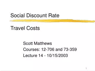
Applications of Simulation Travel Costs. Scott Matthews Courses: 12-706 / 19-702. Admin Issues. No Friday class this week More on HW 4 – removing Q #17. Will show updated grade range Wed (regrades) Today: @RISK tutorial, stochastic dominance Need to specify take-home final plans

E N D
Applications of SimulationTravel Costs Scott Matthews Courses: 12-706 / 19-702
Admin Issues • No Friday class this week • More on HW 4 – removing Q #17. • Will show updated grade range Wed (regrades) • Today: @RISK tutorial, stochastic dominance • Need to specify take-home final plans • Week of Dec 8-12, Two timeslots? • #1: Morning of 8th – 5pm on 10th • #2: Morning of 10th – 5pm on 12th 12-706 and 73-359
@RISK tutorial/simulations • @RISK the “most different” of the plugins in latest version • Please look at the online materials (not just book tutorial) since various things different. • Another current application: • www.fivethirtyeight.com 12-706 and 73-359
Stochastic Dominance “Defined” • A is better than B if: • Pr(Profit > $z |A) ≥ Pr(Profit > $z |B), for all possible values of $z. • Or (complementarity..) • Pr(Profit ≤ $z |A) ≤ Pr(Profit ≤ $z |B), for all possible values of $z. • A FOSD B iff FA(z) ≤ FB(z) for all z 12-706 and 73-359
Stochastic Dominance:Example #1 • CRP below for 2 strategies shows “Accept $2 Billion” is dominated by the other. 12-706 and 73-359
Stochastic Dominance (again) • Chapter 4 (Risk Profiles) introduced deterministic and stochastic dominance • We looked at discrete, but similar for continuous • How do we compare payoff distributions? • Two concepts: • A is better than B because A provides unambiguously higher returns than B • A is better than B because A is unambiguously less risky than B • If an option Stochastically dominates another, it must have a higher expected value 12-706 and 73-359
First-Order Stochastic Dominance (FOSD) • Case 1: A is better than B because A provides unambiguously higher returns than B • Every expected utility maximizer prefers A to B • (prefers more to less) • For every x, the probability of getting at least x is higher under A than under B. • Say A “first order stochastic dominates B” if: • Notation: FA(x) is cdf of A, FB(x) is cdf of B. • FB(x) ≥ FA(x) for all x, with one strict inequality • or .. for any non-decr. U(x), ∫U(x)dFA(x) ≥ ∫U(x)dFB(x) • Expected value of A is higher than B 12-706 and 73-359
FOSD 12-706 and 73-359 Source: http://www.nes.ru/~agoriaev/IT05notes.pdf
Option A Option B FOSD Example 12-706 and 73-359
Second-Order Stochastic Dominance (SOSD) • How to compare 2 lotteries based on risk • Given lotteries/distributions w/ same mean • So we’re looking for a rule by which we can say “B is riskier than A because every risk averse person prefers A to B” • A ‘SOSD’ B if • For every non-decreasing (concave) U(x).. 12-706 and 73-359
Option A Option B SOSD Example 12-706 and 73-359
Area 2 Area 1 12-706 and 73-359
SOSD 12-706 and 73-359
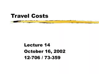
Travel Costs Scott Matthews 12-706 / 19-702
Travel Costs • Time is a valuable commodity (time is $) • Arguably the most valuable • All about opportunity cost • Most major transportation/infrastructure projects built to ‘save travel costs’ • Need to tradeoff project costs with benefits • Ex: new highway that shortens commutes • Differences between ‘travel’ and ‘waiting’ • Waiting time disutility might be orders of magnitude higher than just ‘travel disutility’ • Why? Travelling itself might be fun 12-706 and 73-359
Valuation: Travel Cost Method • Estimate economic use values associated with ecosystems or sites that are used for recreation • changes in access costs for a recreational site • elimination of an existing recreational site • addition of a new recreational site • changes in environmental quality • www.ecosystemvaluation.org/travel_costs.htm 12-706 and 73-359
Travel Cost Method • Basic premise - time and travel cost expenses incurred to visit a site represent the “price” of access to the site. • Thus, peoples’ WTP to visit the site can be estimated based on the number of trips that they make at different travel costs. • This is analogous to estimating peoples’ WTP for a marketed good based on the quantity demanded at different prices. 12-706 and 73-359
Example Case • A site used mainly for recreational fishing is threatened by development. • Pollution and other impacts from this development could destroy the fish habitat • Resulting in a serious decline in, or total loss of, the site’s ability to provide recreational fishing services. • Resource agency staff want to determine the value of programs or actions to protect fish habitat at the site. 12-706 and 73-359
Why Use Travel Cost? • Site is primarily valuable to people as a recreational site. There are no endangered species or other highly unique qualities that would make non-use values for the site significant. • The expenditures for projects to protect the site are relatively low. Thus, using a relatively inexpensive method like travel cost makes the most sense. • Relatively simple compared to other methods 12-706 and 73-359
Options for Method • A simple zonal travel cost approach, using mostly secondary data, with some simple data collected from visitors. • An individual travel cost approach, using a more detailed survey of visitors. • A random utility approach using survey and other data, and more complicated statistical techniques. 12-706 and 73-359
Zonal Method • Simplest approach, estimates a value for recreational services of the site as a whole. Cannot easily be used to value a change in quality of recreation for a site • Collect info. on number of visits to site from different distances. Calculate number of visits “purchased” at different “prices.” • Used to construct demand function for site, estimate consumer surplus for recreational services of the site. 12-706 and 73-359
Zonal Method Steps • 1. define set of zones around site. May be defined by concentric circles around the site, or by geographic divisions, such as metropolitan areas or counties surrounding the site • 2. collect info. on number of visitors from each zone, and the number of visits made in the last year. • 3. calculate the visitation rates per 1000 population in each zone. This is simply the total visits per year from the zone, divided by the zone’s population in thousands. 12-706 and 73-359
Sample Data 12-706 and 73-359
Estimating Costs • 4. calculate average round-trip travel distance and travel time to site for each zone. • Assume Zone 0 has zero travel distance and time. • Use average cost per mile and per hour of travel time, to calculate travel cost per trip. • Standard cost per mile is $0.30. The cost of time is from average hourly wage. • Assume that it is $9/hour, or $.15/minute, for all zones, although in practice it is likely to differ by zone. 12-706 and 73-359
Data 5. Use regression to find relationship between visits and travel costs, e.g. Visits/1000 = 330 – 7.755*(Travel Cost) “a proxy for demand given the information we have” 12-706 and 73-359
Final steps • 6. construct estimated demand for visits with regression. First point on demand curve is total visitors to site at current costs (with no entry fee), which is 1600 visits. Other points by estimating number of visitors with different hypothetical entrance fees (assuming that an entrance fee is valued same as travel costs). Start with $10 entrance fee. Plugging this into the estimated regression equation, V = 330 – 7.755C: 12-706 and 73-359
Demand curve • This gives the second point on the demand curve—954 visits at an entry fee of $10. In the same way, the number of visits for increasing entry fees can be calculated: 12-706 and 73-359
Graph Consumer surplus = area under demand curve = benefits from recreational uses of site around $23,000 per year, or around $14.38 per visit ($23,000/1,600). Agency’s objective was to decide feasibility to spend money to protect this site. If actions cost less than $23,000 per year, the cost will be less than the benefits provided by the site. 12-706 and 73-359
Recreation Benefits • Value of recreation studies • ‘Values per trip’ -> ‘value per activity day’ • Activity day results (Sorg and Loomis 84) • Sport fishing: $25-$100, hunting $20-$130 • Camping $5-$25, Skiing $25, Boating $6-$40 • Wilderness recreation $13-$75 • Are there issues behind these results? 12-706 and 73-359
Value of travel time savings • Many studies seek to estimate VTTS • Can then be used easily in CBAs • Waters, 1993 (56 studies) • Many different methods used in studies • Route, speed, mode, location choices • Results as % of hourly wages not a $ amount • Mean value of 48% of wage rate (median 40) • North America: 59%/42% • Good resource for studies like this: www.vtpi.org 12-706 and 73-359
Government Analyses • DOT (1997): Use % of wage rates for local/intercity and personal/business travel • These are the values we will use in class 12-706 and 73-359 Office of Secretary of Transportation, “Guidance for the Valuation of Travel Time in Economic Analysis”, US DOT, April 1997.
In-and-out of vehicle time 12-706 and 73-359
Income and VTTS • Income levels are important themselves • VTTS not purely proportional to income • Waters suggests ‘square root’ relation • E.g. if income increases factor 4, VTTS by 2 12-706 and 73-359
Introduction - Congestion • Congestion (i.e. highway traffic) has impacts on movement of people & goods • Leads to increased travel time and fuel costs • Long commutes -> stress -> quality of life • Impacts freight costs (higher labor costs) and thus increases costs of goods & services • http://mobility.tamu.edu/ 12-706 and 73-359
Literature Review • Texas Transportation Institute’s 2005 Annual Mobility Report • http://tti.tamu.edu/documents/mobility_report_2005.pdf • 20-year study to assess costs of congestion • Average daily traffic volumes • Binary congestion values • ‘Congested’ roads assumed both ways • Assumed 5% trucks all times/all roads • Assumed 1.25 persons/vehicle, $12/hour • Assumed roadway sizes for 3 classes of roads • Four different peak hour speeds (both ways) 12-706 and 73-359
Results • An admirable study at the national level • In 2003, congestion cost U.S. 3.7 billion hours of delay, 2.3 billion gallons of wasted fuel, thus $63 billion of total cost 12-706 and 73-359
Long-term effects (Tufte?) Uncongested 33% Severe 20% Heavy 14% 12-706 and 73-359
Old / Previous Results • Method changed over time.. • In 1997, congestion cost U.S. 4.3 billion hours of delay, 6.6 billion gallons of wasted fuel, thus $72 billion of total cost • New Jersey wanted to validate results with its own data 12-706 and 73-359
New Jersey Method • Used New Jersey Congestion Management System (NJCMS) - 21 counties total • Hourly data! Much more info. than TTI report • For 4,000 two-direction links • Freeways principal arteries, other arteries • Detailed data on truck volumes • Average vehicle occupancy data per county, per roadway type • Detailed data on individual road sizes, etc. 12-706 and 73-359
Level of Service • Description of traffic flow (A-F) • A is best, F is worst (A-C ‘ok’, D-F not) • Peak hour travel speeds calculated • Compared to ‘free flow’ speeds • A-C classes not considered as congested • D-F congestion estimated by free-peak speed • All attempts to make specific findings on New Jersey compared to national • http://www.njit.edu/Home/congestion/ 12-706 and 73-359
Definitions • Roadway Congestion Index - cars per road space, measures vehicle density • Found per urban area (compared to avgs) • > 1.0 undesirable • Travel Rate Index • Amount of extra time needed on a road peak vs. off-peak (e.g. 1.20 = 20% more) 12-706 and 73-359
Definitions (cont.) • Travel Delay - time difference between actual time and ‘zero volume’ travel time • Congestion Cost - delay and fuel costs • Fuel assumed at $1.28 per gallon • VTTS - used wage by county (100%) • Also, truck delays $2.65/mile (same as TTI) • Congestion cost per licensed driver • Took results divided by licenses • Assumed 69.2% of all residents each county 12-706 and 73-359
Details • County wages $10.83-$23.20 per hour • Found RCI for each roadway link in NJ • Aggregated by class for each county 12-706 and 73-359
New York City RCI result: Northern counties generally higher than southern counties 12-706 and 73-359
TRI result: Northern counties generally higher than southern counties 12-706 and 73-359
Avg annual Delay = 34 hours! Almost a work Week! 12-706 and 73-359
Effects • Could find annual hours of delay per driver by aggregating roadway delays • Then dividing by number of drivers • Total annual congestion cost $4.9 B • Over 5% of total of TTI study • 75% for autos (190 M hours, $0.5 B fuel cost) • 25% for trucks (inc. labor/operating cost) • Avg annual delay per driver = 34 hours 12-706 and 73-359