Download
1 / 22
220 likes | 661 Vues
Examples and SAS introduction: -Violations of the rare disease assumption -Use of Fisher’s exact test January 14, 2004. 1. When can the OR mislead?. General Rule of Thumb: “OR is a good approximation as long as the probability of the outcome in the unexposed is less than 10%”.

E N D
Examples and SAS introduction:-Violations of the rare disease assumption -Use of Fisher’s exact testJanuary 14, 2004
General Rule of Thumb: “OR is a good approximation as long as the probability of the outcome in the unexposed is less than 10%” When is the OR is a good approximation of the RR?
February 25, 1999 Volume 340:618-626 From: “The Effect of Race and Sex on Physicians' Recommendations for Cardiac Catheterization” • Study overview: • Researchers developed a computerized survey instrument to assessphysicians' recommendations for managing chest pain. • Actorsportrayed patients with particular characteristics (race and sex) in scriptedinterviews about their symptoms. • 720 Physicians attwo national meetings viewed a recordedinterview and was given other data about a hypothetical patient.He or she then made recommendations about that patient's care.
February 25, 1999 Volume 340:618-626 From: “The Effect of Race and Sex on Physicians' Recommendations for Cardiac Catheterization”
The Media Reports: “Doctors were only 60 percent as likely to order cardiac catheterization for women and blacks as for men and whites. For black women, the doctors were only 40 percent as likely to order catheterization.” Their results…
Media headlines on Feb 25th, 1999… Wall Street Journal: “Study suggests race, sex influence physicians' care.” New York Times: Doctor bias may affect heart care, study finds.” Los Angeles Times: “Heart study points to race, sex bias.” Washington Post: “Georgetown University study finds disparity in heart care; doctors less likely to refer blacks, women for cardiac test.” USA Today: “Heart care reflects race and sex, not symptoms.” ABC News: “Health care and race”
A closer look at the data… The authors failed to report the risk ratios: RR for women: .847/.906=.93 RR for black race: .847/.906=.93 Correct conclusion: Only a 7% decrease in chance of being offered correct treatment.
Lessons learned: • 90% outcome is not rare! • OR is a poor approximation of the RR here, magnifying the observed effect almost 6-fold. • Beware! Even the New England Journal doesn’t always get it right! • SAS automatically calculates both, so check how different the two values are even if the RR is not appropriate. If they are very different, you have to be very cautious in how you interpret the OR.
Cath No Cath Female 305 55 Male 326 34 360 360 SAS code and outputfor generating OR/RR from 2x2 table
data cath_data; input IsFemale GotCath Freq; datalines; 1 1 305 1 0 55 0 1 326 0 0 34 run; data cath_data; *Fix quirky reversal of SAS 2x2 tables; set cath_data; IsFemale=1-IsFemale; GotCath=1-GotCath; run; proc freq data=cath_data; tables IsFemale*GotCath /measures; weight freq; run;
SAS output Statistics for Table of IsFemale by GotCath Estimates of the Relative Risk (Row1/Row2) Type of Study Value 95% Confidence Limits ƒƒƒƒƒƒƒƒƒƒƒƒƒƒƒƒƒƒƒƒƒƒƒƒƒƒƒƒƒƒƒƒƒƒƒƒƒƒƒƒƒƒƒƒƒƒƒƒƒƒƒƒƒƒƒƒƒƒƒƒƒƒƒƒƒ Case-Control (Odds Ratio) 0.5784 0.3669 0.9118 Cohort (Col1 Risk) 0.9356 0.8854 0.9886 Cohort (Col2 Risk) 1.6176 1.0823 2.4177 Sample Size = 720
Fisher’s “Tea-tasting experiment” (p. 40 Agresti) Claim: Fisher’s colleague (call her “Cathy”) claimed that, when drinking tea, she could distinguish whether milk or tea was added to the cup first. To test her claim, Fisher designed an experiment in which she tasted 8 cups of tea (4 cups had milk poured first, 4 had tea poured first). Null hypothesis: Cathy’s guessing abilities are no better than chance. Alternatives hypotheses: Right-tail: She guesses right more than expected by chance. Left-tail: She guesses wrong more than expected by chance
Milk Tea Milk 3 1 Tea 1 3 Guess poured first Poured First 4 4 Fisher’s “Tea-tasting experiment” (p. 40 Agresti) Experimental Results:
Milk Milk Tea Tea Milk Milk 3 4 1 0 Tea Tea 0 1 4 3 Guess poured first Guess poured first Poured First Poured First 4 4 4 4 Fisher’s Exact Test Step 1: Identify tables that are as extreme or more extreme than what actually happened: Here she identified 3 out of 4 of the milk-poured-first teas correctly. Is that good luck or real talent? The only way she could have done better is if she identified 4 of 4 correct.
Milk Milk Tea Tea Milk Milk 3 4 1 0 Tea Tea 0 1 4 3 Guess poured first Guess poured first Poured First Poured First 4 4 4 4 Fisher’s Exact Test Step 2: Calculate the probability of the tables (assuming fixed marginals)
Step 3: to get the left tail and right-tail p-values, consider the probability mass function: Probability mass function of X, where X= the number of correct identifications of the cups with milk-poured-first: “right-hand tail probability”: p=.243 “left-hand tail probability” (testing the null hypothesis that she’s systematically wrong): p=.986
Milk Tea Milk 3 1 Tea 1 3 4 4 SAS code and outputfor generating Fisher’s Exact statistics for 2x2 table
data tea; input MilkFirst GuessedMilk Freq; datalines; 1 1 3 1 0 1 0 1 1 0 0 3 run; data tea; *Fix quirky reversal of SAS 2x2 tables; set tea; MilkFirst=1-MilkFirst; GuessedMilk=1-GuessedMilk;run; proc freq data=tea; tables MilkFirst*GuessedMilk /exact; weight freq;run;
SAS output Statistics for Table of MilkFirst by GuessedMilk Statistic DF Value Prob ƒƒƒƒƒƒƒƒƒƒƒƒƒƒƒƒƒƒƒƒƒƒƒƒƒƒƒƒƒƒƒƒƒƒƒƒƒƒƒƒƒƒƒƒƒƒƒƒƒƒƒƒƒƒ Chi-Square 1 2.0000 0.1573 Likelihood Ratio Chi-Square 1 2.0930 0.1480 Continuity Adj. Chi-Square 1 0.5000 0.4795 Mantel-Haenszel Chi-Square 1 1.7500 0.1859 Phi Coefficient 0.5000 Contingency Coefficient 0.4472 Cramer's V 0.5000 WARNING: 100% of the cells have expected counts less than 5. Chi-Square may not be a valid test. Fisher's Exact Test ƒƒƒƒƒƒƒƒƒƒƒƒƒƒƒƒƒƒƒƒƒƒƒƒƒƒƒƒƒƒƒƒƒƒ Cell (1,1) Frequency (F) 3 Left-sided Pr <= F 0.9857 Right-sided Pr >= F 0.2429 Table Probability (P) 0.2286 Two-sided Pr <= P 0.4857 Sample Size = 8