Download
1 / 26
260 likes | 391 Vues
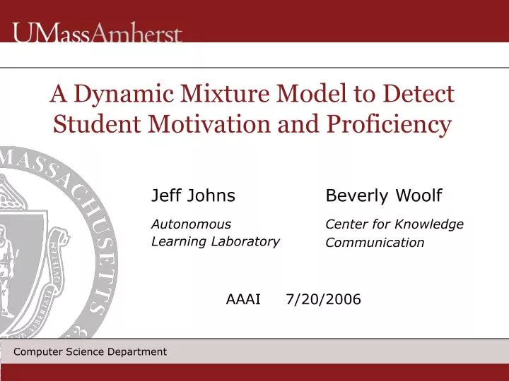
A Dynamic Mixture Model to Detect Student Motivation and Proficiency. Jeff Johns Autonomous Learning Laboratory. Beverly Woolf Center for Knowledge Communication. AAAI 7/20/2006. Agenda. Problem Statement Proposed Model Results Conclusions and Future Work. Problem Statement.

E N D
A Dynamic Mixture Model to Detect Student Motivation and Proficiency Jeff Johns Autonomous Learning Laboratory Beverly Woolf Center for Knowledge Communication AAAI 7/20/2006
Agenda • Problem Statement • Proposed Model • Results • Conclusions and Future Work
Problem Statement • Background • Develop a machine learning component for a geometry tutoring system used by high school students (SAT, MCAS) • Focus on estimating the “state” of a student, which is then used for selecting an appropriate pedagogical action • Problem • Currently using a model to estimate student ability, but… • Students appear unmotivated in ~30% of problems • Solution • Explicitly model motivation (as a dynamic variable) and student proficiency in a single model
Wayang Outpost, a Geometry Tutor wayang.cs.umass.edu
Low Student Motivation • Example: Actual data from a student performing 12 problems (green = correct, red = incorrect) • Problems are of roughly equal difficulty • Student appears to perform well in beginning and worse toward the end • Conclusion: The student’s proficiency is average … 1 2 3 4 5 6 7 8 9 10 11 12
Low Student Motivation • However, we come to a different conclusion when considering the student’s response time! 50 40 30 Time (s) To First Response 20 10 0 … 1 2 3 4 5 6 7 8 9 10 11 12
Low Student Motivation • Conclusion: Poor performance on the last five problems is due to low motivation (not proficiency) 50 40 30 Time (s) To First Response Use observed data to infer motivation! Student is unmotivated 20 10 0 … 1 2 3 4 5 6 7 8 9 10 11 12
Low Student Motivation • Opportunity for intelligent tutoring systems to improve student learning by addressing motivation • This issue is being dealt with on a larger scale by the educational assessment community • Wise & Demars 2005. Low Examinee Effort in Low-Stakes Assessment: Potential Problems and Solutions. Educational Assessment.
Agenda • Problem Statement • Proposed Model • Results • Conclusions and Future Work
Combined Model • Jointly estimate proficiency and motivation in a single model Item Response Theory Model Hidden Markov Model Combined Model + = • Used to estimate • student proficiency • (continuous and • static variable) • Used to estimate • student motivation • (discrete and • dynamic variable) • More accurately • estimate proficiency • by accounting for • motivation • Design appropriate • interventions based • on motivation • estimate
Item Response Theory (IRT) • Random Variables • Ui {correct, incorrect} student response to problem i • k student ability • ~ MVN(0, I) (assume k=1) • Joint Probability = P() P(Ui | ) • Problems are assumed independent • Ability () is a static variable • P(Ui | ) is modeled using an item characteristic curve n i=1 U1 U2 U3 … Un
Item Characteristic Curve • Two parameter (a&b) logistic curve relating ability () to the probability of a correct response • Prob. of correct response = [1 + exp(-a(–b))]-1 Discrimination Parameter (a) Difficulty Parameter (b)
Hidden Markov Model (HMM) • A HMM is used to capture a student’s changing behavior (level of motivation) M1 M2 … Mn H1 H2 … Hn
Combined Model • New edges (in red) change the conditional probability of a student’s response: P(Ui | , Mi) M1 M2 … Mn Motivation (Mi) affects student response (Ui) H1 H2 … Hn U1 U2 … Un
How Motivation Affects Response • P(Ui | , Mi) viewed as a mixture of behaviors (Mi) Mi = Unmotivated (many hints) Mi = Unmotivated (quick guess) Mi = Motivated
How Motivation Affects Response • P(Ui | , Mi) viewed as a mixture of behaviors (Mi) Mi = Unmotivated (many hints) Mi = Unmotivated (quick guess) Mi = Motivated P(Ui | , Mi=motivated) = [1 + exp(-a(–b))]-1 IRT describes behavior
How Motivation Affects Response • P(Ui | , Mi) viewed as a mixture of behaviors (Mi) Mi = Unmotivated (many hints) Mi = Unmotivated (quick guess) Mi = Motivated P(Ui | , Mi=motivated) = [1 + exp(-a(–b))]-1 IRT describes behavior P(Ui | , Mi=unmotivated) = constant Performance is independent of ability!
Parameter Estimation • Uses an Expectation-Maximization algorithm to estimate parameters • M-Step is iterative, similar to the Iterative Reweighted Least Squares (IRLS) algorithm • Model consists of discrete and continuous variables • Integral for the continuous variable is approximated using a quadrature technique • Only parameters not estimated • P(Ui | , Mi=unmotivated-guess) = 0.2 • P(Ui | , Mi=unmotivated-hint) = 0.02
Agenda • Problem Statement • Proposed Model • Results • Conclusions and Future Work
Modeling Ability and Motivation • Combined model does not decrease the ability estimate when the student is unmotivated
Modeling Ability and Motivation • Combined model does not decrease the ability estimate when the student is unmotivated • Combined model separates ability from motivation (IRT model lumps them together)
Experiments: Five-Fold Cross-Validation • Data: 400 high school students, 70 problems, a student finished 32 problems on average • Train the Model • Estimate parameters • Test the Model • For each student, for each problem: • Estimate and P(Mi) via maximum likelihood • Predict P(Mi+1) given HMM dynamics • Predict Ui+1. Does it match actual Ui+1? • Compare combined model vs. just an IRT model
Results • Combined model achieved 72.5% cross-validation accuracy versus 72.0% for the IRT model • Gap is not statistically significant • Opportunities for improving the accuracy of the combined model • Longer sequences (per student) • Better model of the dynamics, P(Mi+1 | Mi)
Agenda • Problem Statement • Proposed Model • Results • Conclusions and Future Work
Conclusions • Proposed a new, flexible model to jointly estimate student motivation and ability • Not separating ability from motivation conflates the two concepts • Easily adjusted for other tutoring systems • Combined model achieved similar accuracy to IRT model • Online inference in real-time • Implemented in Java; ran it in one high school in May ’06
Future Work • Improve the combined model’s accuracy • Tests with simulated students • Better modeling of the dynamics, P(Mi+1 | Mi) • Create interventions to engage unmotivated students Intervention 1 Intervention 2 Mi+1 Mi Unmotivated ??? Intervention 3