Download
1 / 18
180 likes | 344 Vues
Sparse Recovery Using Sparse (Random) Matrices. Piotr Indyk MIT. Joint work with: Radu Berinde, Anna Gilbert, Howard Karloff, Martin Strauss and Milan Ruzic. Goal of this talk. “Stay awake until the end”. Ax. A. =. x. x. x*. k=2.

E N D
Sparse Recovery Using Sparse (Random) Matrices Piotr Indyk MIT Joint work with: Radu Berinde, Anna Gilbert, Howard Karloff, Martin Strauss and Milan Ruzic
Goal of this talk “Stay awake until the end”
Ax A = x x x* k=2 Linear Compression(learning Fourier coeffs, linear sketching, finite rate of innovation, compressed sensing...) • Setup: • Data/signal in n-dimensional space : x E.g., x is an 1000x1000 image n=1000,000 • Goal: compress x into a “sketch” Ax , where A is a m x n “sketch matrix”, m << n • Requirements: • Plan A: want to recover x from Ax • Impossible: undetermined system of equations • Plan B: want to recover an “approximation” x* of x • Sparsity parameter k • Want x* such that ||x*-x||p C(k) ||x’-x||q ( lp/lq guarantee ) over all x’ that are k-sparse (at most k non-zero entries) • The best x* contains k coordinates of x with the largest abs value • Want: • Good compression (small m) • Efficient algorithms for encoding and recovery • Why linear compression ?
destination source Linear compression: applications • Data stream algorithms (e.g. for network monitoring) • Efficient increments: A(x+) = Ax + A • Single pixel camera [Wakin, Laska, Duarte, Baron, Sarvotham, Takhar, Kelly, Baraniuk’06] • Pooling, Microarray Experiments [Kainkaryam, Woolf], [Hassibi et al], [Dai-Sheikh, Milenkovic, Baraniuk]
Constructing matrix A • Choose encoding matrix Aat random (the algorithms for recovering x* are more complex) • Sparse matrices: • Data stream algorithms • Coding theory (LDPCs) • Dense matrices: • Compressed sensing • Complexity/learning theory (Fourier matrices) • “Traditional” tradeoffs: • Sparse: computationally more efficient, explicit • Dense: shorter sketches • Goal: the “best of both worlds”
“state of art” Scale: Excellent Very Good Good Fair Prior and New Results
dense vs. sparse • Restricted Isometry Property (RIP) *- sufficient property of a dense matrix A: is k-sparse ||||2 ||A||2 C ||||2 • Holds w.h.p. for: • Random Gaussian/Bernoulli: m=O(k log (n/k)) • Random Fourier: m=O(k logO(1) n) • Consider random m x n 0-1 matrices with d ones per column • Do they satisfy RIP ? • No, unless m=(k2)[Chandar’07] • However, they can satisfy the following RIP-1 property [Berinde-Gilbert-Indyk-Karloff-Strauss’08]: is k-sparse d (1-) ||||1 ||A||1 d||||1 • Sufficient (and necessary) condition: the underlying graph is a ( k, d(1-/2) )-expander * Other (weaker) conditions exist, e.g., “kernel of A is a near-Euclidean subspace of l1”. More later.
Expanders • A bipartite graph is a (k,d(1-))-expander if for any left set S, |S|≤k, we have |N(S)|≥(1-)d |S| • Constructions: • Randomized: m=O(k log (n/k)) • Explicit: m=k quasipolylog n • Plenty of applications in computer science, coding theory etc. • In particular, LDPC-like techniques yield good algorithms for exactly k-sparse vectors x [Xu-Hassibi’07, Indyk’08, Jafarpour-Xu-Hassibi-Calderbank’08] N(S) d S m n
Proof: d(1-/2)-expansion RIP-1 • Want to show that for any k-sparse we have d (1-) ||||1 ||A ||1 d||||1 • RHS inequality holds for any • LHS inequality: • W.l.o.g. assume |1|≥… ≥|k| ≥ |k+1|=…= |n|=0 • Consider the edges e=(i,j) in a lexicographic order • For each edge e=(i,j) define r(e) s.t. • r(e)=-1 if there exists an edge (i’,j)<(i,j) • r(e)=1 if there is no such edge • Claim 1: ||A||1 ≥∑e=(i,j) |i|re • Claim 2: ∑e=(i,j) |i|re ≥ (1-) d||||1 d m n
Matching Pursuit(s) A x*-x Ax-Ax* • Iterative algorithm: given current approximation x* : • Find (possibly several) i s. t. Ai “correlates” with Ax-Ax* . This yields i and z s. t. ||x*+zei-x||p << ||x* - x||p • Update x* • Sparsify x* (keep only k largest entries) • Repeat • Norms: • p=2 : CoSaMP, SP, IHTetc (dense matrices) • p=1 : SMP, this paper (sparse matrices) • p=0 : LDPC bit flipping (sparse matrices) = i i
Sequential Sparse Matching Pursuit • Algorithm: • x*=0 • Repeat T times • Repeat S=O(k) times • Find i and zthat minimize* ||A(x*+zei)-b||1 • x* = x*+zei • Sparsify x* (set all but k largest entries of x* to 0) • Similar to SMP, but updates done sequentially A i N(i) Ax-Ax* x-x* * Set z=median[ (Ax*-Ax)N(i) ]. Instead, one could first optimize (gradient) i and then z [ Fuchs’09]
SSMP: Running time • Algorithm: • x*=0 • Repeat T times • For each i=1…n compute* zi that achieves Di=minz ||A(x*+zei)-b||1 and store Di in a heap • Repeat S=O(k) times • Pick i,z that yield the best gain • Update x* = x*+zei • Recompute and store Di’ for all i’ such that N(i) and N(i’) intersect • Sparsify x* (set all but k largest entries of x* to 0) • Running time: T [ n(d+log n) + k nd/m*d (d+log n)] = T [ n(d+log n) + nd (d+log n)] = T [ nd (d+log n)] A i Ax-Ax* x-x*
x a2 a1 x a1 a2 Supports of a1anda2have small overlap (typically) SSMP: Approximation guarantee • Want to find k-sparse x* that minimizes ||x-x*||1 • By RIP1, this is approximately the same as minimizing ||Ax-Ax*||1 • Need to show we can do it greedily
Experiments 256x256 SSMP is ran with S=10000,T=20. SMP is ran for 100 iterations. Matrix sparsity is d=8.
Conclusions • Even better algorithms for sparse approximation (using sparse matrices) • State of the art: can do 2 out of 3: • Near-linear encoding/decoding • O(k log (n/k)) measurements • Approximation guarantee with respect to L2/L1 norm • Questions: • 3 out of 3 ? • “Kernel of A is a near-Euclidean subspace of l1” [Kashin et al] • Constructions of sparse A exist [Guruswami-Lee-Razborov, Guruswami-Lee-Wigderson] • Challenge: match the optimal measurement bound • Explicit constructions Thanks! This talk