Download
1 / 21
210 likes | 306 Vues
steady state impacts in inverse model parameter optimization.

E N D
steady state impacts in inverse model parameter optimization Carvalhais, N., Reichstein, M., Seixas, J., Collatz, G.J., Pereira, J.S., Berbigier, P., Carrara, A., Granier, A., Montagnani, L., Papale, D., Rambal, S., Sanz, M.J., and Valentini, R.(2008), Implications of the carbon cycle steady state assumption for biogeochemical modeling performance and inverse parameter retrieval, Global Biogeochem. Cycles, 22, GB2007, doi:10.1029/2007GB003033.
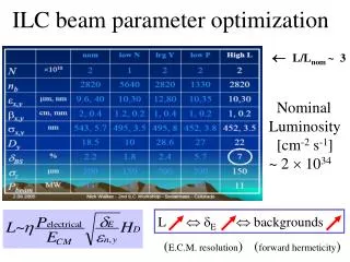
motivation / goals • CASA model parameter optimization • spin-up routines force soil C pools estimates • impacts of the steady state in: • model performance • parameter estimates / constraints • propagation of C fluxes estimates uncertainties for the Iberian Peninsula
the CASA model Potter et al., 1993
Fix Steady State Relaxed Steady State approach to relax the steady state approach • inclusion of a parameter that relaxed the steady state approach: η Cns = Css ∙η
experiment design • significance of each parameter: • removing one parameter at a time; • alternatives to η: • replacing by : • soil C turnover rates; • extra parameters on NPP and Rh temperature sensitivity. • Levenberg-Marquardt least squares optimization
site selection and data • CARBOEUROPE-IP: • 10 Sites • optimization constraints: NEP • model drivers: • site meteorological data; • remotely sensed fAPAR and LAI; • different temporal resolutions
adding η effect of ηin optimization IT-Non [sink: 542gC m-2 yr-1]
determinants of parameter variability: ANOVA site parameter vector temporal resolution site x parameter vector site x temporal resolution parameter vector x temporal resolution
r2: 0.76; α < 0.001 what drives η?
model performance improvements model performance in relaxed > fixed steady state assumptions.
relaxed relaxed ↓Rh ↑NPP fixed fixed Topt Topt Bwε Bwε Q10 Q10 Aws Aws ε* ε* differences in parameter estimates and constraints P/P SE/SE
relaxed fixed measurements total soil C pools
steady state approach impacts • model performance • relaxed > fixed • parameter estimates • biases • parameter uncertainties • relaxed < fixed • soil C pools estimates • relaxed closer to measurements
spatial simulations • Iberian Peninsula • optimized parameters per site: • optimization: naïve bootstrap approach • no assumption on parameters distribution • GIMMS NDVIg : 8km, biweekly; • parameter propagation per PFT: • estimating NEP / NPP / Rh
relaxed fixed relaxed - fixed spatial impacts : NPP 1991
seasonality : NPP : IP relaxedversusfixed
iav : NEP : IP relaxedversusfixed
seasonality and iav : IP (relax – fix) / fix
remarks • biases in optimized parameters lead to significant differences in flux estimates: seasonality and iav • uncertainties propagation show significant reductions under relaxed steady state approaches • impacts in data assimilation schemes