Download

1 / 37
370 likes | 541 Vues
The Microarchitecture Level. Chapter 4. A Design with Prefetching: Mic-2. The IFU reduces the path length of the average instruction. it eliminates the main loop entirely, since the end of each instruction simply branches to the next instruction.

E N D
The Microarchitecture Level Chapter 4
A Design with Prefetching: Mic-2 • The IFU reduces the path length of the average instruction. • it eliminates the main loop entirely, since the end of each instruction simply branches to the next instruction. • it avoids tying up the ALU incrementing PC. • it reduces the path length when a 16-bit index is calculated. • Figures 4-29 and 4-30 show Mic-2 and the corresponding microcode, respectively. • IADD instruction • There is no need to go to Main1 • When the IFU sees that MBR1 has been referenced in iadd3, its internal shift register pushes everything to the right and reloads MBR1 and MBR2 • It also makes a transition to a state one lower than its current one. • If the new state is 2, the IFU starts fetching a word from memory. • All this is in hardware. • For overall performance, the gain for more common instructions is what really counts.
A Design with Prefetching: Mic-2 • Figure 4-29. The data path for Mic-2.
A Design with Prefetching: Mic-2 Figure 4-30. The microprogram for the Mic-2 (part 1 of 3).
A Design with Prefetching: Mic-2 Figure 4-30. The microprogram for the Mic-2 (part 2 of 3).
A Design with Prefetching: Mic-2 Figure 4-30. The microprogram for the Mic-2 (part 3 of 3).
A Pipelined Design: The Mic-3 • The cycle time can be decreased by bringing in more parallelism into the machine. • There are three major components to the actual data path cycle: • The time to drive the selected registers onto the A and B buses • The time for the ALU and shifter to do their work • The time for the results to get back to the registers and be stored. • In fig. 4-31 we show a new three-bus architecture, including the IFU, but with three additional latches (registers), one inserted in the middle of each bus. • The registers partition the data path into distinct parts that can now operate independently of one another. • Now it takes three clock cycles to use the data path. • The latches serve the following purpose: • Speed up the clock as the maximum delay is shorter • All parts of the data path can be used during every cycle.
A Pipelined Design: The Mic-3 Figure 4-31. The three-bus data path used in the Mic-3
A Pipelined Design: The Mic-3 Label Operations Comments swap1 MAR=SP-1; rd Read 2nd word from stack; set MAR to SP swap2 MAR = SP Prepare to write new 2nd word swap3 H=MDR; wr Save new TOS; write 2nd word to stack swap4 MDR = TOS copy old TOS to MDR swap5 MAR = SP-1; wr Write old TOS to 2nd place on stack swap6 TOS = H; goto(MBR1) Update TOS • Figure 4-32. The Mic-2 code for SWAP. • We assume that memory operation takes one cycle. • The implementation of SWAP for Mic-2 is shown below: • The data path now requires three cycles to operate, and we call each of these steps as microsteps.
A Pipelined Design: The Mic-3 • Figure 4-33. The implementation of SWAP on the Mic-3.
A Pipelined Design: The Mic-3 • We observe that a new microinstruction is started on every clock cycle except in cycle 3. • This is because MDR is not available until the start of cycle 5. • True dependence or RAW dependence: When a microstep cannot be started as it depends on the result of the previous microstep which is not available. • Stalling: Stopping to wait for a needed value from the previous step • Mic-3 takes more cycles than Mic-2 but runs faster • Assume: Mic-3 cycle time is T nsec • Mic-3 requires 11T nsec, and Mic-2 takes 6 cycles at 3T = 18T
A Pipelined Design: The Mic-3 • Figure 4-34. Graphical illustration of how a pipeline works.
A Seven-Stage Pipeline: Mic-4 • Figure 4-35. The main components of the Mic-4.
A Seven-Stage Pipeline: Mic-4 • The IFU feeds the incoming byte stream to a new component: decoding unit. • The decoding unit has an internal ROM indexed by IJVM opcode. • Each entry contains two parts: • Length of that IJVM instruction • Index into another ROM • The IJVM instruction length is used to allow the decoding unit to parse the incoming byte stream into instructions, so it always knows which bytes are opcodes and which are operands. • The index maps to the micro-operation ROM in the queuing unit. • The queuing unit contains some logic plus two internal tables, one in ROM and one in RAM. • The ROM contains the microprogram, with each IJVM instruction having some number of consecutive entries, called micro-operations • The entries must be in order, so wide_iload2 branching to iload2 in Mic-2 are not allowed.
A Seven-Stage Pipeline: Mic-4 • The micro-operations are similar to the microinstructions except that the NEXT_ADDRESS and JAM fields are absent, and a new encoded field is needed to specify the A bus input. • Two new bits are also provided: Final and Goto. • The Finalbit represents the last micro-operation of each IJVM micro-operation sequence. • The Goto bit is set to mark micro-operations that are conditionalmicrobranches. • Such micro-operations have a different format from the normal micro-operations, consisting of the JAM bits and an index into the micro-operation ROM. • The queuing unit receives a micro-operation ROM index from the decoding unit. • It then looks up the micro-operation and copies it into an internal queue. • It copies all the micro-operations until the last one that has the Final bit set.
A Seven-Stage Pipeline: Mic-4 • If a micro-operation has the Goto bit OFF, and there is still space in the queue, queuing unit sends acknowledgement signal to the decoding unit. • When the decoding unit sees the acknowledgement, it sends the index of the next IJVM instruction to the queuing unit. • These micro-operations feed the MIRs, which send the signals out to control the data path. • Since all the fields in a micro-operation are not active at the same time, four independent MIRs have been introduced in Mic-4. • AT the start of each cycle (w time), MIR3 is copied to MIR4, MIR2 is copied to MIR3, MIR1 is copied to MIR2 and MIR1 is loaded with a fresh micro-operation from the micro-operation queue. • Then each MIR puts out its control signals in different clock cycles. • The A and B fields from MIR1 are used to select the registers that drive the A and B latches in the first cycle, and so on for other MIRs.
A Seven-Stage Pipeline: Mic-4 • Some IJVM instructions, such as IFLT, need to conditionally branch based on, say the N bit. • To deal with microbranch, the Goto bit is checked in the micro-operation. • If the Goto bit is set, the queuing unit does not send an acknowledgement to the decoding unit, until the microbranch has been resolved. • It is possible that some IJVM instructions beyond the branch have already been fed into the decoding unit ( but not into queuing unit), since an acknowledgement was not received from the queuing unit. • Special hardware and mechanisms are required to clean up the mess and get back on track. • Mic-4 is a highly pipelined design with seven stages and far more complicated hardware than Mic-1
A Seven-Stage Pipeline: Mic-4 • Figure 4-36. The Mic-4 pipeline. • The Mic-4 automatically prefetches a stream of bytes from memory, decodes them into IJVM instructions, converts them to a sequence of micro-operations using a ROM, and queues them for use as needed. • First three stages of the pipeline can be tied to the data path clock if desired, but there will not always be work to do. • For example, the IFU can certainly not feed a new IJVM opcode to the decoding unit on every clock cycle because IJVM instructions take several cycles to execute and the queue would rapidly overflow. • Each MIR controls a different part of the data path and thus different microsteps. • The pipelined design makes the steps small and thus clock frequency high.
Improving Performance • Two types of improvement • implementation improvements and • architectural improvements • Implementation improvements: are ways of building a new CPU or memory to make the system run faster without changing the architecture. • One way to improve the implementation is to use a faster clock • Architectural improvements: adding new instructions or registers, so that old programs will continue to run on the new models. • For full performance gain, the software must be changed, or at least recompiled with a new compiler that takes advantage of the new features.
Cache Memory (1) • Multiple caches improve both bandwidth and latency. • Split cache: separate cache for instructions and data. • Level 2 cache, may reside between the instruction and data caches and main memory. • The CPU chip itself contains a small instruction cache and a small data cache, typically 16 KB to 64 KB. • A typical size for the L2 cache is 512 KB to 1 MB. • Figure 4-37. A system with three levels of cache.
Cache Memory (2) • Spatial locality: memory locations with addresses numerically similar to a recently accessed memory location are likely to be accessed in the near future. • Temporal locality: recently accessed memory locations are accessed again. • for example, memory locations near the top of the stack, or instructions inside a loop • Main memory is divided up into fixed-size blocks called cache lines. • Cache line: consists of 4 to 64 consecutive bytes. • With a 32-byte line size, line 0 is bytes 0 to 31, line 1 is bytes 32 to 63, and so on.
Direct-Mapped Caches (1) With a 32-byte cache line size, the cache can hold 2048 entries of 32 bytes or 64 KB in total. Each cache entry consists of three parts: Valid bit indicates whether there is any valid data in this entry Tag field with unique, 16-bit value identifying corresponding line of memory from which data came Data field contains copy of data in memory. Holds one cache line of 32 bytes. • Figure 4-38. (a) A direct-mapped cache. (b) A 32-bit virtual address.
Direct-Mapped Caches (2) TAG field corresponds to Tag bits stored in cache entry. LINE field indicates which cache entry holds corresponding data, if present. WORD field tells which word within a line is referenced. BYTE field usually not used, but if only single byte is requested, tells which byte within word is needed.
Direct-Mapped Caches (3) • CPU produces a memory address; hardware extracts the 11 LINE bits from the address to index into the 2048 cache entries. • Cache hit: if entry is valid, and if TAG field of the memory address and the Tag field in cache entry are same, the cache entry holds the word being requested. • Only the word actually needed is extracted from the cache entry. The rest of the entry is not used. • Cache miss: if the cache entry is invalid or the tags do not match, the needed entry is not present in the cache • In this case, the 32-byte cache line is fetched from memory and stored in the cache entry, replacing what was there. • Write back to main memory if the existing cache entry has been modified.
Direct-Mapped Caches (4) • Up to 64 KB of contiguous data can be stored in the cache. • However, two lines that differ in their address by precisely 65,536 bytes or any integral multiple of that number cannot be stored in the cache at the same time (because they have the same LINE value). • If a program accesses data at location X and next executes an instruction that needs data at location X + 65,536, the second instruction will force the cache entry to be reloaded, overwriting what was there. • If this happens often enough, it can result in poor behavior. • The worst-case behavior of a cache is worse than if there were no cache at all.
Set-Associative Caches (1) • If a program using Direct-mapped cache heavily uses words at addresses 0 and at 65,536, there will be constant conflicts. • Each reference potentially evicts the other one from the cache. • A solution is to allow two or more lines in each cache entry. • n-way set-associative cache: a cache with n possible entries for each address • Figure 4-39. A four-way set-associative cache.
Set-Associative Caches (2) • Replacement policy: Least Recently Used (LRU) • keeps an ordering of each set of locations that could be accessed from a given memory location. • Whenever any of the present lines are accessed, it updates the list, marking that entry the most recently accessed. • To replace an entry, the one at the end of the list—the least recently accessed—is the one discarded. • High-associativity caches do not improve performance much over low-associativity caches under most circumstances. • When a processor writes a word, and the word is in the cache, it obviously must either update the word or discard the cache entry. • updating the copy in main memory can be deferred until later, when the cache line is ready to be replaced by the LRU algorithm.
Set-Associative Caches (3) • write through: immediately updating the entry in main memory. • This approach is generally simpler to implement and more reliable, since the memory is always up to date—helpful, for example, if an error occurs and it is necessary to recover the state of the memory. • Unfortunately, it also usually requires more write traffic to memory, • Write deferred, or write back: more sophisticated implementations • what if a write occurs to a location that is not currently cached? • write allocation: most designs that defer writes to memory tend to bring data into the cache on a write miss • Most designs employing write through, tend not to allocate an entry on a write; this option complicates an otherwise simple design.
Branch Prediction (1) Figure 4-40. (a) A program fragment. (b) Its translation to a generic assembly language. • Pipelining works best on linear code • The fetch unit can just read in consecutive words from memory and send them off to the decode unit in advance of their being needed. • Programs are not linear code sequences. • They are full of branch instructions. • In the example below, two of the five instructions are branches, one of these, BNE, is a conditional branch
Branch Prediction (2) • Unconditional branch • instruction decoding occurs in the second stage • the fetch unit has to decide where to fetch from next before it knows what kind of instruction it just got. • Only one cycle later can it learn that it just picked up an unconditional branch, and by then it has already started to fetch the instruction following the unconditional branch. • As a consequence, a substantial number of pipelined machines have the property that the instruction following an unconditional branch is executed, even though logically it should not be. • The position after a branch is called a delay slot. • An optimizing compiler inserts a NOP instruction in the delay slot. • Doing so keeps the program correct, but makes it bigger and slower
Branch Prediction (3) • Conditional branch • the fetch unit does not know where to read from until much later in the pipeline • Early pipelined machines just stalled until it was known whether the branch would be taken or not. • most machines predict whether the branch is going to be taken or not. • A simple way: assume that all backward conditional branches will be taken and that all forward ones will not be taken. • backward branches are frequently located at the end of a loop. • Some forward branches occur when error conditions are detected in software. • Errors are rare, so most of the branches associated with them are not taken. • Of course, there are plenty of forward branches not related to error handling
Branch Prediction (4) • branch is predicted incorrectly • allow instructions fetched after a predicted conditional branch to execute until they try to change the machine’s state (e.g., storing into a register). • Instead of overwriting the register, the value computed is put into a (secret) scratch register and only copied to the real register after it is known that the prediction was correct. • The second way is to record the value of any register about to be overwritten (e.g., in a secret scratch register), so the machine can be rolled back to the state it had at the time of the mispredicted branch. • Both solutions are complex and require industrial-strength bookkeeping to get them right.
Dynamic Branch Prediction (1) Figure 4-41. (a) 1-bit branch history. (b) 2-bit branch history. (c) Mapping between branch instruction address, target address. • One approach is for the CPU to maintain a history table (in special hardware), in which it logs conditional branches as they occur, so they can be looked up when they occur again. • In (a) below the history table contains one entry for each conditional branch instruction.
Dynamic Branch Prediction (2) • several ways to organize the history table – as in cache • A machine with 32-bit instructions that are word aligned will have low-order 2 bits of each memory address 00 • With a direct-mapped history table containing 2n entries, the low-order n + 2 bits of a branch instruction target address can be extracted and shifted right 2 bits. • Use n-bit number as an index into the history table; check if address stored there matches the address of the branch. • no need to store the low-order n + 2 bits, just the tag • If hit, use prediction bit to predict the branch. • If wrong tag is present or entry is invalid, a miss occurs, just as with a cache. • In this case, the forward/backward branch rule can be used.
Dynamic Branch Prediction (3) • A two-way, four-way, or n-way associative entry can be used for conflicts, just as in cache. • A Problem: when a loop is finally exited, the branch at the end will be mispredicted, and will change the bit in the history table to indicate a future prediction of ‘‘no branch.’’ • The next time the loop is entered, the branch at the end of the first iteration will be predicted wrong. • Solution: give the table entry a second chance. • With this method, the prediction is changed only after two consecutive incorrect predictions. • requires two prediction bits, one for what the branch is ‘‘supposed’’ to do, and one for what it did last time
Dynamic Branch Prediction (4) Figure 4-42. A 2-bit finite-state machine for branch prediction. • The leftmost bit of the state is the prediction and the rightmost bit is what the branch did last time. • A design that keeps track of 4 or 8 bits of history is also possible. • FSMs are very widely used in all aspects of hardware design.
End Chapter 4