Download
1 / 28
300 likes | 797 Vues
Solution Methods. Overview. Properties of Numerical Solution Methods FVM and FEM solution methods Characteristics of solution algorithms Equations solvers Underrelaxation Convergence. Numerical Solution Methods (1). The important components of a numerical solution method are:

E N D
Overview • Properties of Numerical Solution Methods • FVM and FEM solution methods • Characteristics of solution algorithms • Equations solvers • Underrelaxation • Convergence
Numerical Solution Methods (1) • The important components of a numerical solution method are: 1. Mathematical model of flow • e.g. equations of motion- unsteady and steady, compressible and incompressible, 2D and 3D, turbulence, etc. 2. Discretization Method • Approximation of the differential equations by a system of algebraic equations • Finite Difference Method (FDM) • Finite Volume Method (FVM) • Finite Element Method (FEM) 3. Coordinate system • cartesian or cylindrical, curvilinear orthogonal and non-orthogonal coordinate systems
Numerical Solution Methods (2) 4. Numerical Grid • The solution domain is subdivided by the grid. The algebraic conservation equations for the variables are computed on a finite number of control volumes or elements in the domain. • Types of Grids • Structured grids • Multi-block-structured grids • Unstructured grids Unstructured surface grid for vehicle aerodynamic analysis. 5. Finite Approximations • Discretizing the solution domain gives rise to errors from the approximation of the continuous differential functions • FDM - approximate the derivatives through the Taylor series expansion • FVM - approximate the surface and volume integrals • FEM - choose weighting functions
Numerical Solution Methods (3) 6. Solution Criteria and Convergence Criteria • This is the topic of this lecture • Methods of solving the system of algebraic equations • The nonlinear nature of the governing equations requires an iterative solution method. Convergence criteria determine when to terminate the iterative process. Accuracy and efficiency are considered.
Properties of Solution Methods • Consistency • Stability • Convergence • Conservation • Boundedness • Realizability • Accuracy
N n j E P W e w s i S FVM - Solution Algorithms • The discretized form of the governing conservation equations can be written as: • where nb denotes the cell neighbors of cell P • In a 2D structured grid, the face P has fourneighbors (E,W,N,S). In a 3D grid, a cell hassix neighbors. • In an unstructured grid, the number of neighbors depends on the cell shape and mesh topology. • The above algebraic equation is written for each transport variable, that is, velocity, temperature, species concentration and turbulence quantities.
FVM - Solution Algorithms • The solution of the Navier-Stokes equations is complicated by the lack of an independent equation for pressure. Pressure is linked to all three momentum equations • The pressure-velocity coupling algorithm SIMPLE (Semi-Implicit Pressure Linked Equations), and it’s variants, are used. • Concept: • the momentum equations are used to compute velocity • a pressure equation is derived from the continuity equation • a discrete pressure correction equation is derived from the discrete forms of the pressure and momentum equations • the pressure correction equation is updated with pressure and a mass flux balance through a mass correction
Finite Volume Solution Methods • The Finite Volume Solution method can either use a “segregated” or a “coupled” solution procedure. • The solution procedure of each method is the same.
Update properties. Solve momentum equations (u, v, w velocity). Solve pressure-correction (continuity) equation. Update pressure, face mass flow rate. Solve energy, species, turbulence, and other scalar equations. Converged? No Yes Stop Segregated Solution Procedure
No Yes Coupled Solution Procedure Update properties. Solve continuity, momentum, energy, and species equations simultaneously. Solve turbulence and other scalar equations. Converged? Stop
No Yes Stop Unsteady Solution Procedure • Same procedure for segregated and coupled solvers: Execute segregated or coupled procedure, iterating to convergence Update solution values with converged values at current time Requested time steps completed? Take a time step
FVM - Linear Equation Solvers • Consider the system of algebraic equations for variable f • The above system of equations is arranged in a matrix and solved iteratively. • For a structured grid, the coefficient matrix is banded. Special line-by-line iterative techniques such as the Line Gauss-Seidel (LGS) method may be used. • LGS method involves solving the equations in a “line” simultaneously. • The equations are set-up in a tri-diagonal matrix solved via Gaussian elimination • For an unstructured grid, no line structure exists. Point-iterative methods are used, e.g., the Point Gauss-Seidel (PGS) technique. • LGS/PGS locally reduce errors but can miss long-wavelength errors. Multigrid acceleration will speed up the LGS/PGS convergence.
Marching direction sweeping direction Flow Values from previous sweep Line to be solved Values from previous iteration FVM - Line Gauss-Seidel (LGS) Method • The LGS method is used on structured grids and involves the following steps: • simultaneously solve the equations in the sweep direction • march to next row or column
FVM - The Multigrid Solver • The LGS and PGS solvers both transmit the influence of near-neighbors effectively and are less effective at transmitting the influence of far away grid points and boundaries, thereby, slowing convergence. • “Multigrid” solver accelerates convergence for: • Large number of cells • Large cell aspect ratios • x/y > 20 • Large differences in thermal conductivity • Such as in conjugate heat transfer • General concept of multigrid is the same for structured and unstructured grids, although the implementation is different.
coarse grid level 1 coarse grid level 2 original grid The Multigrid Concept (1) • Multigrid solver uses a sequence of grids going from fine to coarse. • Influence of boundaries and far-away points more easily transmitted to interior on coarse meshes than on fine meshes. • In coarse meshes, grid points are closer together in the computational space and have fewer computational cells between any two spatial locations. • Fine meshes give more accurate solutions.
corrections coarse mesh fine mesh summed equations (or volume-averaged solution) The Multigrid Concept (2) • The solutions on the coarser meshes is used as a starting point for solutions on the finer meshes. • Coarse-mesh solution contains influence of boundaries and far neighbors. • These effects felt more easily on coarse mesh. • Accelerates convergence on fine mesh. • Final solution obtained for original (fine) mesh. • Coarse mesh calculations: • only accelerates convergence • do not change final answer
FVM - Under-relaxation • Equation set being solved is non-linear. • Equation for one variable may depend on other variables, e.g., • Temperature • Mass fraction • For stability the change in a variable fp value from iteration to iteration is reduced by an “under-relaxation” factor, : • For example, an under-relaxation of 0.2 restricts the change in P to 20% of the computed change of for one iteration.
FVM - Residuals and Convergence • At convergence: • All discrete conservation equations (momentum, energy, etc.) are obeyed in all cells to a specified tolerance. • The solution no longer changes with additional iterations. • Mass, momentum, energy and scalar balances are obtained. • “Residuals” measure imbalance (or error) in conservation equations. • Residual at point P is defined as: • An overall measure of the residual in the domain is: • Residuals can be scaled relative to the starting residual
Finite Element Solution Methods • We seek a solution to the equation of the form: K(u) u = F • A solution method is made up of two parts • Algorithm: solution organization scheme • Equation solver: solves linear system of equations • We shall consider two algorithms and two equation solvers
FEM Algorithms and Equation Solvers • Algorithms: • fully-coupled • segregated • Equation solvers: • Gaussian elimination • Iterative methods: • non-symmetric equation systems • symmetric equation systems (pressure eqns.)
Fully-Coupled Algorithm (1) • The most common solution scheme is the so-called Newton-Raphson iteration, or Newton’s method for short • First, re-write the equation as: R(u) = K(u) u - F • Using a Taylor series expansion and some further manipulations, we arrive at:
Fully-Coupled Algorithm (2) • Advantages: • converges very rapidly • Disadvantages: • requires good initial guess • calculation of J-1(ui) is expensive • Alternatives: • Modified Newton-Raphson: evaluate J-1(ui) only once • Quasi-Newton: update J-1(ui) in a simple manner graphic representation of Newton’s method
Segregated Algorithm (1) • K(u) u = F is never formed • Rather, it is decomposed into a set of decoupled equations: • Kuu - Cxp = fuu momentum equation • Kvv - Cyp = fv v momentum equation • CxTu + CyTv = 0 continuity equation • KTT = fT energy (scalar) equation • No explicit equation for pressure! • Replace continuity equation with Poisson-type pressure matrix equation (derived from manipulating discretized momentum and continuity eqn’s) • The pressure can be calculation in a number of ways
Segregated Algorithm (2) • Pressure projection method • given the current values of u, v and T, obtain an approximate pressure bo solving a discrete pressure equation • relax the pressure, i.e.: • using pnew, solve the momentum equations and energy equation • using the newly computed velocities, solve for the pressure correction, Dp • adjust the velocity field (so that it obeys the incompressibility constraint) using Dp • Advantage: less memory use • Disadvantage: more iterations Each equation set can be solved iteratively (inner iteration) or simulaneously (Gaussian elimination) uvpT outer iteration
Equation Solvers • Iterative • Non-symmetric equation systems: • Conjugate gradient squared • GMRES • Symmetric equation systems (pressure): • Conjugate gradient • Conjugate residual • Gaussian elimination
Underrelaxation • Two forms are used • explicit (similar to FVM approach) • carries some “history” forward • used with fully-coupled method • also used for pressure in segregated method • implicit • alters the weighting term for matrix diagonal • used for other equations (not pressure) with segregated method
Convergence • Various quantities can be used to judge convergence of an FEM solution • The more commonly used are: • Relative change in solution between iterations ||Ui - Ui-1|| / ||Ui|| < tolerance • Relative numerical accuracy (R is residual vector) ||Ri|| / ||R0|| < tolerance