Download
1 / 39
400 likes | 650 Vues
Discrete Random Variables – Outline. Two kinds of random variables Discrete Continuous 2. Describing a DRV 3. Expected value of a DRV 4. Variance of a DRV 5. Examples. Two kinds of random variables. Discrete (DRV). Outcomes have countable values (can be listed)

E N D
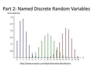
Discrete Random Variables – Outline • Two kinds of random variables • Discrete • Continuous 2. Describing a DRV 3. Expected value of a DRV 4. Variance of a DRV 5. Examples Discrete Random Variables
Two kinds of random variables • Discrete (DRV) • Outcomes have countable values (can be listed) • E.g., # of people in this room • Possible values can be listed: might be …51 or 52 or 53… Discrete Random Variables
Two kinds of random variables • Discrete • Continuous (CRV) • Not countable • Consists of points in an interval • E.g., time till coffee break • CRVs are the subject of next week’s lecture Discrete Random Variables
Describing a DRV • We begin by defining the DRV of interest • For example, if our experiment is to toss a fair coin twice, we could define the variable X as the # of heads that occurs in those two tosses. Discrete Random Variables
Describing a DRV • To describe a DRV, we specify the possible values and their respective probabilities. • For the coin-toss experiment, we have: PossibleProbability values 0 .25 1 .5 2 .25 Notes: P(x) ≥ 0, ∀x. ∑p(x) = 1.0 Discrete Random Variables
Expected value of a DRV • We can compute the average or “expected value” of a DRV • This is the average value of X that we would find over many repetitions of the experiment • It is a theoretical quantity based on the possible values and their probabilities Discrete Random Variables
Expected value of a DRV • Example experiment: two tosses of a fair coin • DRV: X = # of heads that occur • Expected value of X: the mean # of heads that would occur over many repetitions of the experiment. Discrete Random Variables
Expected value of a DRV Expected value: μ = E(x) = ∑[x * p(x)] Variance: σ2 = ∑[(x – μ)2 * p(x)] Note: σ = √σ2 Discrete Random Variables
Expected Value of a DRV For the coin toss: PossibleProbability values 0 ¼ 1 ½ 2 ¼ μ = (0 * ¼) + (1 * ½) + (2 * ¼) = 1 σ2 = [(0-1)2 * ¼] + [(1-1)2 * ½] + [(2-1)2 * ¼] = ½ Discrete Random Variables
Example 1 12 candidates apply for positions in a local law firm (8 men and 4 women). The firm decides that they only have enough money to hire 3 of the applicants. They decide to give each applicant an aptitude test and hire the 3 with the highest scores. Assume that law aptitude is randomly distributed in the population and that, on average, there are no differences between women and men. Let the random variable X be the number of women who score in the top 3 on the aptitude test. What is the distribution of X? Discrete Random Variables
Example 1 First, what is the DRV? • X = # of women who score in the top 3 on the law aptitude test. Discrete Random Variables
Example 1 Second, what are the possible outcomes? 0, 1, 2, and 3 Do you see why? Discrete Random Variables
Example 1 Next, what are the probabilities of these outcomes? The question says that law aptitude is randomly distributed with no sex difference. Therefore, the probability that we get 0 women in the top 3 is: 8 4 3 0 12 3 ( ) ( ) ) ( Discrete Random Variables
Example 1 # of ways of choosing 0 women out of 4 8 4 3 0 12 3 ( ) ( ) ( ) Total # of ways of choosing 3 candidates out of 12 # of ways of choosing 3 men out of 8 Discrete Random Variables
( ) ( ) ( ) Example 1 The question says that law aptitude is randomly distributed with no sex difference. Therefore, the probability that we get 0 women in the top 3 is: 8 4 3 0 = 56 = .254 12 220 3 Discrete Random Variables
Example 1 We compute the probabilities of other outcomes similarly. For P(x =1): 8 4 2 1 = 112 = .509 12 220 3 ( ) ( ) ( ) Discrete Random Variables
Example 1 P(X = 2): 8 4 1 2 = 48 = .218 12 220 3 ( ) ( ) ) ( Discrete Random Variables
Example 1 P(X = 3): 8 4 0 3 = 4 = .018 12 220 3 ( ) ( ) ) ( Discrete Random Variables
Example 1 X P(X) 0 .254 1 .509 2 .218 3 .018 This is how we present the distribution. These are the values that X can take These are the probabilities for each value of X Discrete Random Variables
Example 2 In the game GAMBLE, a player flips a coin and the game ends when the first head occurs or after the fifth flip. However, the nature of the coin’s bias changes over successive flips, such that the true ratio of heads to tails is n:1 for a given flip, where n is the ordinal position of a given flip in the series of flips (for example, the ratio of heads to tails for the third flip would be 3:1). The player loses $20 if the game ends after the first flip. The player wins (n X $10) if the game ends after any of flips 2 through 5. Let X be the amount of money that can be won or lost playing the game one time (losses are represented by negative amounts). What is the Expected Value of X ? Discrete Random Variables
Example 2 First, what are the possible outcomes? X = amount of money that can be won or lost when playing the game once. Recall that the player loses $20 (X = -20) if the game ends on the first flip. Possible values (in dollars): X = -20, 20, 30, 40, or 50 Discrete Random Variables
Example 2 Next, what has to happen to produce each of these outcomes? We need to specify that in order to work out the probabilities. XWhat has to happen -20 H 20 T, H 30 T, T, H 40 T, T, T, H 50 T, T, T, T, H or T, T, T, T, T Discrete Random Variables
Example 2 • Now, what are the probabilities? • To answer, we have to specify the probabilities of H on each flip – because the question tells us these probabilities keep changing. Discrete Random Variables
Example 2 Flip #Ratio H:TP(H) 1 1:1 .5 2 2:1 .67 3 3:1 .75 4 4:1 .80 5 5:1 .83 2:1 means that out of every 3 flips, 2 will be heads and 1 will be tails – so we get P(heads) = 2/3 (= .67) Remember that the ratio of heads to tails is n:1 for the nth trial Discrete Random Variables
Example 2 We can now work out the probabilities: X P(X) -20 .5 20 .5*.67 30 .5*.33*.75 40 .5*.33*.25*.80 50 .5*.33*.25*.20*.83 + .5*.33*.25*.20*.17 This is P(heads) for flip #1 This is P(tails) for flip #2 Discrete Random Variables
Example 2 X P(X) -20 .5 20 .335 30 .12375 40 .033 50 .00825 ΣP(X) = 1.00 Discrete Random Variables
Example 2 We’re not finished yet – the question asks: “What is the Expected Value of X?” µ = (-20)*.5 + (20)*.335 + (30)*.12375) + (40)*.033 + (50)*(.00825) = 2.145 (Now we’re finished!) Discrete Random Variables
Example 3 3. In a local basketball league, when a person is fouled they get to shoot two free throws. Over the years of playing in the league, Beth has calculated that every time she takes two free throws, she makes her first free throw 60% of the time. If she makes her first free throw, she makes the second one 70% of the time. If she misses the first one, she makes the second one only 40% of the time. Discrete Random Variables
Example 3 a) Let X be the # of free throws that Beth makes when she goes to the free throw line to shoot two free throws. What is the probability distribution for X? First, what are the possible outcomes? Beth could make 0, 1, or 2 free throws. Discrete Random Variables
Example 3 Secondly, how might these outcomes be achieved? OutcomeFirst throwSecond throw 0 Miss Miss 1 Hit Miss 1 Miss Hit 2 Hit Hit Discrete Random Variables
Example 3 Let’s define: Event A = Beth makes the free throw on the first attempt Event B = Beth makes the free throw on the second attempt We are given P(A) = .60 P(B│A) = .70 P(B’│A) = .30 P(B│A’) = .40 Discrete Random Variables
Example 3 Compute: For X = 0 P(A’B’) = P(A’) * P(B’│A’) = .60 * .40 = .24 For X = 1 P(AB’) = P(A) * P(B’│A) = .60 * .30 = .18 Discrete Random Variables
Example 3 For X = 1 P(A’B) = P(A’) * P(B│A’) = .40 * .40 = .16 Thus, P(X = 1) = .18 + .16 = .34 For X = 2 P(AB) = P(A) * P(B│A) = .60 * .70 = .42 Discrete Random Variables
Example 3 X P(X) 0.24 1.34 2.42 μ = Σ(x* p(x)) = 0 *.24 + 1*.34 + 2*.42 = 1.18 σ2 = Σ[(x-μ)2 * p(x)] = [(0-1.18)2 * .24] + [(1-1.18)2 * .34] + [(2-1.18)2 * .42] = .627 σ = √.627 = .792 Discrete Random Variables
Example 3 b) In the next game, Beth gets fouled twice. On both occasions, she gets to shoot two free throws. This is equivalent to taking a sample of size 2 from the distribution you created in part a) above. Let Y = the total # of free throws Beth makes in those 2 opportunities to shoot two free throws. What is the probability distribution of Y? Discrete Random Variables
Example 3 First, what are the possible outcomes? “a sample of size 2” means 2 trips to the free throw line, with two throws on each trip. Therefore, possible outcomes for Y are 0, 1, 2, 3, and 4. Discrete Random Variables
Example 3 Secondly, what the respective probabilities of these outcomes? To answer this question, we have to think about how each outcome might arise… Discrete Random Variables
Example 3 Y # hits first trip # hits second trip 0 0 0 1 0 1 1 1 0 2 2 0 2 0 2 2 1 1 3 2 1 3 1 2 4 2 2 P(Y = 1) will have two components P(Y = 2) will have three components Discrete Random Variables
Example 3 – the probability distribution YComponent probabilitiesP(Y) 0 .24 * .24 .0576 1 (.24*.34) + (.34*.24) .1632 2 (.42*.24) + (.24*.42) + (.34*.34) .3172 3 (.34*.42) + (.42*.34) .2856 4 (.42*.42) .1764 Σ= 1.000 Discrete Random Variables