Download
1 / 37
370 likes | 483 Vues
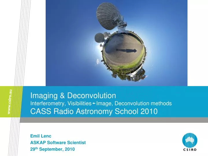
Emil Lenc ASKAP Software Scientist 29 th September, 2010. Imaging & Deconvolution Interferometry, Visibilities➛Image, Deconvolution methods CASS Radio Astronomy School 2010. Interferometry concepts.

E N D
Emil Lenc • ASKAP Software Scientist • 29th September, 2010 Imaging & DeconvolutionInterferometry, Visibilities➛Image, Deconvolution methodsCASS Radio Astronomy School 2010
Interferometry concepts • Visibility = coherence between average electric fields across FOV of two antennas separated by a baseline. • Long baseline • Delay variation of many wavelengths across field, narrow fringe pattern, extended sources average out - high resolution. • Short baseline • Delay variation across field less than a wavelength, wide fringe pattern, flux from extended sources adds up - low resolution. CSIRO. Imaging & Deconvolution Radio Astronomy School 2010
Fourier basics Image plane uv plane F(s) SmallF(as) Hermitian (F(s)=F(-s)*) Convolve F*G Phase Gradient Add (F+G) Rotate f(x) Large f(x/a) Real Multiply f g Shiftf(x+a) Add f+g Rotate Fourier Transform 3 CSIRO. Imaging & Deconvolution Radio Astronomy School 2010
The uv plane • Visibilities have coordinates: u,v • Baselines trace out arcs in uv plane • Earth rotation fills the plane • Hybrid array with N-S baselines fills plane quicker (6-8h) • For low frequency long N-S baselines need to consider w-term. East-west array CSIRO. Imaging & Deconvolution Radio Astronomy School 2010
Regular calibrator scans Image plane and uv plane Flagged data Missing hour angles Missing of flagged baselines uv plane Image plane CSIRO. Imaging & Deconvolution Radio Astronomy School 2010
Fourier pairs CSIRO. Imaging & Deconvolution Radio Astronomy School 2010
The dirty beam • Dirty beam = PSF (Point Spread Function) = • Response to unit point source at field centre = FT of uv coverage. CSIRO. Imaging & Deconvolution Radio Astronomy School 2010
The uv plane features • Dense rings • Baselines – tracks in uv plane • Low level in between rings • Gaps in coverage, missing information • Hole in centre • No information on low 'spatial frequencies', i.e., no info on large scale structure • Outer boundary • No info on small scale structure – resolution limit • Ways to fill the uv plane • Add single dish data • Multiple configurations (needs more time) • Multi-frequency synthesis CSIRO. Imaging & Deconvolution Radio Astronomy School 2010
Multi-frequency synthesis (MFS) • As uv coordinates are measured in wavelengths, another way of filling the Fourier plane is to observe at multiple wavelengths simultaneously. • Standard for ATCA continuum (up to 2048 x 1 MHz channels per band) • Potential for great improvement of coverage at 6cm and 12mm • Need to take extra care as source emission can vary with frequency. CSIRO. Imaging & Deconvolution Radio Astronomy School 2010
Image plane Partially cleaned image Dirty beam or PSF Note extended source and sources outside field CSIRO. Imaging & Deconvolution Radio Astronomy School 2010
Imaging decisions • Some decisions best made at proposal or observing stage, some at processing stage • Field of view (FOV) • Based on primary beam size, mosaicing (multiple fields) • 20cm – 33' beam, 3mm – 30'' beam • may need to image larger field to remove side-lobes from distant sources • Shortest baseline determines largest structure we can image well • Resolution/tapering, cell size (>2 pixels/beam) • Longest baseline determines limit to resolution • Many observations do NOT want maximum resolution because sensitivity to extended structure is low: “object is resolved out” • Many short baseline configurations: EW352, H75 • often elect not to include long baselines (e.g., deselect CA06 ) • adds high frequency ripple to image with mostly short baselines CSIRO. Imaging & Deconvolution Radio Astronomy School 2010
Imaging decisions 6 cm observation of Circinus A in EW352 configuration uv coverage with no MFS uv coverage MFS with CABB CSIRO. Imaging & Deconvolution Radio Astronomy School 2010
Imaging decisions • Weighting scheme • Uniform (minimises side-lobe level) • Natural (minimises noise level) • Robust (optimal combination of above two with a “sliding scale”) Uniform Beam: 7”x5” Sensitivity: 1.45 Robust = 0.5 Beam: 8”x6.5” Sensitivity: 1.16 Robust = 1.0 Beam: 9.6”x7.5” Sensitivity: 1.06 Natural Beam: 12”x8” Sensitivity: 1.0 CSIRO. Imaging & Deconvolution Radio Astronomy School 2010
Imaging decisions • Continuum • combine channels (ATCA Pre-CABB continuum obs. had 32x 4MHz channels) • possibly combine multiple centre frequencies (MFS) • e.g. for increased sensitivity at 12mm combine 21 GHz and 23 GHz observations. • Creates single output image at ‘average’ frequency • Line • Check velocity frame, Doppler correction • Specify spectral resolution & velocity range • Creates output image cube – an image for each frequency channel (RA,Dec,Vel) • CABB (Compact Array Broadband Backend) • changes the standard division between continuum & line • Standard continuum observation: 2x2 GHz bandwidth (1MHz channels) • Line – 4 zoom bands e.g, 1 MHz BW, 2048 channels (16 zooms in future) • All simultaneously! CSIRO. Imaging & Deconvolution Radio Astronomy School 2010
Imaging decisions • Polarisation • Choice of stokes I,Q,U,V if observing all combinations (XX,XY,YX,YY) • Pre-CABB spectral line modes often only offered XX,YY, for full stokes I sensitivity, at half the data rate. • CABB now offers full stokes even for spectral line modes. • Time averaging • You may want to average data online (10s -> 30s) for low frequency spectral line work to reduce data volume • Drawbacks: • Interference spikes may affect more data • Phase instability may cause decorrelation • Wide field imaging may be affected (smearing of sources at large distances from phase-centre) CSIRO. Imaging & Deconvolution Radio Astronomy School 2010
Some details • Imaging uses FFT – works on sampled data • Need to grid the uv data (choice of gridding methods) • Specify gridding convolution function • Suppresses aliasing • Tapering (gaussian taper applied to vis weights) • Another form of weighting to influence beam size, useful to match beam size with other observations • Non-coplanar baselines (e.g.VLA at low frequency) • Small field approximation fails, use e.g., w-projection imaging • Generally not an issue with the ATCA. CSIRO. Imaging & Deconvolution Radio Astronomy School 2010
Beyond the dirty image ... • Calibration and Fourier transform get us to the best possible dirty image • To improve things further we want to: • Remove the side-lobes of the dirty beam from our image (clean…) • Dirty Image = Sky convolved with dirty beam • Need a deconvolution procedure • Linear? • Non-linear? CSIRO. Imaging & Deconvolution Radio Astronomy School 2010
Linear deconvolution • Noise properties are well understood • Generally non-iterative and computationally cheap • Used for e.g., de-blurring photos • But • It does a very poor job • Rarely useful in practical radio interferometry – zeroes in F[B] • Linear deconvolution is fundamentally unable to extrapolate/interpolate unmeasured spatial frequencies. CSIRO. Imaging & Deconvolution Radio Astronomy School 2010
Non-linear deconvolution • A good non-linear deconvolution algorithm is one that picks plausible (‘invisible’) distributions to fill the unmeasured parts of the Fourier plane. • Need to make assumptions to get a realistic estimate • Main assumption: Real sky does NOT look like typical dirty beam • Rings, spokes, negative regions, etc. : all very unlikely • Different algorithms make different assumptions: • CLEAN (pixel based), Point-source fitting • Sky is mostly empty, with occasional peaks • Works well for field with point sources, poor for extended emission • MEM (Maximum Entropy Method) - pixel based • Sky is uniform (& positive) • Works well for very extended sources, poor for point sources • Scale-sensitive algorithms: multi-scale CLEAN, Asp CLEAN, source-fitting • Sky consists of bounded, overlapping, regions of emission CSIRO. Imaging & Deconvolution Radio Astronomy School 2010
CLEAN • Original version by Högbom (1974) • Purely image based • Later versions (Clark, Cotton-Schwab, SDI) add FFT speedups, model visibility subtraction and try to cope with extended emission • Algorithm: • Find position of highest peak in image – assume this is a point source • Subtract a fraction of this peak (‘gain factor’) using a scaled dirty beam at this position • Add model component to list • Go to 1, unless prescribed flux limit or iteration limit reached CSIRO. Imaging & Deconvolution Radio Astronomy School 2010
Restoring the image • After deconvolution we are left with a residual image • Noise • Weak source structure below the CLEAN cutoff limit • Side-lobes of faint and extended sources • Restored Image • Take residual image • Add point components convolved with gaussian fit to central peak of dirty beam • Resulting image is best guess of real sky with measurement noise • Avoids ‘super-resolution’ of component model CSIRO. Imaging & Deconvolution Radio Astronomy School 2010
CLEAN example 1 1, 5, 10, 20, 50, 100, 200, 500, and 1000 CLEAN Components Restored Model: 5 point sources + 1 Gaussian Point: 1,0.5,0.25,0.1,0.01 Jy Gaussian: 0.1Jy, 10”x10” Residual CSIRO. Imaging & Deconvolution Radio Astronomy School 2010
CLEAN example 2 1, 10, 100, 1000, 10000, 100000 CLEAN Components CLEAN model Restored image True sky Dirty image CSIRO. Imaging & Deconvolution Radio Astronomy School 2010
CLEAN strength and weaknesses • CLEAN is good for fields with many compact sources • Effect of defects (RFI, source variability etc.) is generally very local • CLEAN works poorly for very extended objects: • Slow (too many faint point components needed) • Corrugation instability. • CLEAN poorly estimates broad structure (short spacings) -“negative bowl” effect. • CLEAN’s procedural definition makes it difficult to analyse. • But, convergence of Högbom clean was proven under certain conditions (Schwarz,1978) • more data points than clean components, ‘regular beam’ • Clark CLEAN prone to diverge for large iteration numbers (>105) • extend size of beam patch or use Högbom CLEAN instead CSIRO. Imaging & Deconvolution Radio Astronomy School 2010
CLEAN cell size Pixel-centred source Pixel-offset source CSIRO. Imaging & Deconvolution Radio Astronomy School 2010
CLEAN cell size Cell size = beam/6 Cell size = beam/12 Cell size = beam/3 Effect of CLEAN performed on a single 1 Jy source that is not pixel-centred using different cell sizes. CSIRO. Imaging & Deconvolution Radio Astronomy School 2010
MEM • MEM – Maximum Entropy Method • Tries to find the ‘smoothest’ image that is consistent with the data • Image with lowest ‘information content’ for given total flux • No data → flat image • Define smoothness via the ‘entropy’ H • H=-∑kIk ln(Ik/Mke), Ik=pixel k in the image • Use of logarithm enforces positivity constraint • negative sidelobe suppression • Mk is the prior image - a flat default image can be used, but a good low resolution image, if available, is better • Data constraints are added via χ2 of data-model CSIRO. Imaging & Deconvolution Radio Astronomy School 2010
MEM 25 iterations of MEMFinal image = Converged solution Dirty image MEM restored image Final MEM model CSIRO. Imaging & Deconvolution Radio Astronomy School 2010
MEM strengths and weaknesses • In MEM it is easy to add multiple constraints • e.g. information from overlapping fields – mosaicing • Single dish image added to interferometer data • Works well for extended images • Can be much faster than CLEAN for extended structure • Tends to fail for point sources embedded in extended emission (remove those first) • Easier to analyse mathematically • More sensitive to data defects (calibration problems etc) • Effect of errors not localised, may affect convergence • Current implementation does not consider spectral effects. • Care must be taken when using wide-band data e.g. CABB CSIRO. Imaging & Deconvolution Radio Astronomy School 2010
Scale sensitive methods • Both CLEAN and MEM work on single pixels • No inherent notion of source size • When we look at an image we identify a collection of sources of different sizes – makes physical sense too • Adjacent pixels in an image are NOT independent • Resolution limit • Intrinsic source size • e.g. Gaussian source covering 100 pixels can be represented by only 5 parameters instead of 100. • Scale sensitive algorithms try to capture this extra information about a ‘plausible sky’ • Reduces number of degrees of freedom in solution • Separation of signal and noise easier CSIRO. Imaging & Deconvolution Radio Astronomy School 2010
Scale sensitive methods • SDI Clean (Steer-Dewdney-Ito) • One of the early attempts to make CLEAN cope with extended structure • Subtracts scaled beam from a patch of pixels around each peak found • Multi-resolution CLEAN (Wakker-Schwarz) • Make images at 2-4 different resolutions, clean lowest resolution first, then clean residuals at higher resolution • Combined model sensitive to all scales with greatly decreased number of iterations • Multi-scale CLEAN (Cornwell-Holdaway) • Similar, but cleans all scales simultaneously – more robust • Find peak across all image • Remove fraction of peak at that scale from all images • Add corresponding ‘blob’ to model • Iterate until we reach the noise level in all images • Adapted to work with large bandwidths (MSMFS) by modelling spectra for each pixel (using multiple terms if required). CSIRO. Imaging & Deconvolution Radio Astronomy School 2010
Scale sensitive methods • Asp-CLEAN • Decompose image into a set of Adaptive Scale Pixels • pixel → Asp / pixels → Aspen (Bhatnagar & Cornwell, 2004). • Similar to previous methods, but important change: • Components (Aspen) are not fixed once they are in the model • Parameters (flux, size, position) can be updated in subsequent iterations • Algorithm: • 1. Find the peak at a number of scales, pick dominant scale • 2. Take new Aspen, combine with selected Aspen found in earlier iterations – set of ‘active Aspen’ (the ones likely to change) • 3. Fit the set of active Aspen to the data (expensive step). • 4. If termination criterion not met, goto 1. • 5. Smooth with the clean-beam. Add residuals. CSIRO. Imaging & Deconvolution Radio Astronomy School 2010
Asp-CLEAN example (Adaptive Scale Pixel) Model Sky uv Plane Residual CSIRO. Imaging & Deconvolution Radio Astronomy School 2010
Miriad algorithms • Multi-resolution Clean is available in AIPS. • MS-CLEAN and MSMFS-Clean are available in CASA.Asp-CLEAN hasn’t made it into a reduction package yet. • FISTA (Fast Iterative Shrinkage-Thresholding Algorithm) • Uses compressive sampling techniques. • looks promising, still under development, characterisation and testing. • Very fast but unclear how well it responds to noise and calibration errors. CSIRO. Imaging & Deconvolution Radio Astronomy School 2010
Common errors in image plane • Problems remaining after deconvolution • (grating) rings <=> uv tracks • Improve by calibrating slowly varying gain and phase • Radial spokes <=> short times • Improve by calibrating fast varying gain and phase • 'Fuzzy' sources <=> outer tracks bad • decorrelation/bad phase errors (common at high frequency) CSIRO. Imaging & Deconvolution Radio Astronomy School 2010
VRI • VRI, the Virtual Radio Interferometer • Type vri in searchbox on ATNF website • http://www.narrabri.atnf.csiro.au/astronomy/vri.html • Lets you experiment with Fourier transforms and ATCA configurations CSIRO. Imaging & Deconvolution Radio Astronomy School 2010
Acknowledgements • Mark Wierenga 2003/2006/2008 lecture • Bob Sault 2003 lecture • Sanjay Bhatnagar 2006 lecture (NRAO) CSIRO. Imaging & Deconvolution Radio Astronomy School 2010