Download

1 / 38
380 likes | 409 Vues
Topic 11: Aggregate Demand II (chapter 11, Mankiw). Context. Chapter 9 introduced the model of aggregate demand and supply. Chapter 10 developed the IS-LM model, the basis of the aggregate demand curve. In Chapter 11, we will use the IS-LM model to

E N D
Topic 11: Aggregate Demand II (chapter 11, Mankiw)
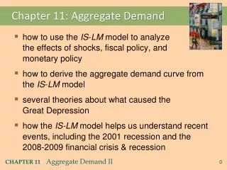
Context • Chapter 9 introduced the model of aggregate demand and supply. • Chapter 10 developed the IS-LM model, the basis of the aggregate demand curve. • In Chapter 11, we will use the IS-LM model to • see how policies and shocks affect income and the interest rate in the short run when prices are fixed • derive the aggregate demand curve • explore various explanations for the Great Depression
LM r IS Y Equilibrium in the IS-LMModel The IScurve represents equilibrium in the goods market. r1 The LMcurve represents money market equilibrium. Y1 The intersection determines the unique combination of Y and rthat satisfies equilibrium in both markets.
LM r r2 r1 IS2 IS1 Y1 Y2 Y 2. 1. 3. An increase in government purchases 1.IScurve shifts right causing output & income to rise. 2. This raises money demand, causing the interest rate to rise… 3. …which reduces investment, so the final increase in Y
LM r r2 1. 2. r1 1. IS2 IS1 Y1 Y2 Y 2. 2. A tax cut Because consumers save (1MPC) of the tax cut, the initial boost in spending is smaller for T than for an equal G… and the IS curve shifts by …so the effects on r and Y are smaller for a T than for an equal G.
LM1 r LM2 r1 r2 IS Y2 Y1 Y Monetary Policy: an increase in M 1. M > 0 shifts the LMcurve down(or to the right) 2. …causing the interest rate to fall 3. …which increases investment, causing output & income to rise.
Shocks in the IS-LM Model ISshocks: exogenous changes in the demand for goods & services. Examples: • stock market boom or crash change in households’ wealth C • change in business or consumer confidence or expectations I and/or C
Shocks in the IS-LM Model LMshocks: exogenous changes in the demand for money. Examples: • a wave of credit card fraud increases demand for money • more ATMs or the Internet banking reduce money demand
CASE STUDYThe U.S. economic slowdown of 2001 ~What happened~ 1. Real GDP growth rate 1994-2000: 3.9% (average annual) 2001: 1.2% 2. Unemployment rate Dec 2000: 4.0% Dec 2001: 5.8%
CASE STUDYThe U.S. economic slowdown of 2001 ~Shocks that contributed to the slowdown~ 1. Falling stock prices (dotcom bubble) From Aug 2000 to Aug 2001: -25% Week after 9/11: -12% 2. The terrorist attacks on 9/11 • increased uncertainty • fall in consumer & business confidence Both shocks reduced spending and shifted the IS curve left.
CASE STUDYThe U.S. economic slowdown of 2001 ~The policy response~ 1. Fiscal policy • large long-term tax cut, immediate $300 tax rebate checks • spending increases:aid to New York City & the airline industry,war on terrorism 2. Monetary policy • Fed lowered its Fed Funds rate target 11 times during 2001, from 6.5% to 1.75% • Money growth increased, interest rates fell
What is the Fed’s policy instrument? What the newspaper says:“the Fed lowered interest rates by one-half point today” What actually happened:The Fed conducted expansionary monetary policy to shift the LM curve to the right until the interest rate fell 0.5 points. The Fed targets the Federal Funds rate: it announces a target value, and uses monetary policy to shift the LM curve as needed to attain its target rate.
IS-LM and Aggregate Demand • So far, we’ve been using the IS-LMmodel to analyze the short run, when the price level is assumed fixed. • However, a change in P would shift the LMcurve and therefore affect Y. • The aggregate demand curve(introduced in chap. 9 ) captures this relationship between P and Y
r P LM(P2) LM(P1) r2 r1 IS Y Y P2 P1 Deriving the AD curve Intuition for slope of ADcurve: P (M/P) LMshifts left r I Y Y1 Y2 AD Y2 Y1
P r LM(M1/P1) LM(M2/P1) r1 r2 IS Y Y Y2 Y1 P1 AD2 AD1 Y1 Y2 Monetary policy and the AD curve The Fed can increase aggregate demand: M LMshifts right r I Y at each value of P
r P LM r2 r1 IS2 IS1 Y Y Y2 Y1 P1 AD2 AD1 Y1 Y2 Fiscal policy and the AD curve Expansionary fiscal policy (G and/or T ) increases agg. demand: T C IS shifts right Y at each value of P
IS1 IS2 LM r 2 2’ LM’ 1 Y1 Y2 Y2’ Policy Effectiveness Fiscal policy is effective (Y will rise much) when: LM flatter As the rise in G raises Y, the increase in money demand does not raise r much: so investment is not crowded out as much.
2’ Y2’ Policy Effectiveness Monetary policy is effective (Y will rise much) when: IS flatter As a rise in M lowers the interest rate (r), investment rises more in response to the fall in r, so output rises more. r IS LM1 LM2 1 2 IS’ Y1 Y2
IS-LM and AD-AS in the short run & long run Recall from Chapter 9: The force that moves the economy from the short run to the long run is the gradual adjustment of prices. In the short-run equilibrium, if then over time, the price level will rise fall remain constant
LRAS r P LM(P1) IS1 IS2 Y Y LRAS SRAS1 P1 AD1 AD2 The SR and LR effects of an IS shock A negative ISshock shifts ISand ADleft, causing Y to fall.
LRAS r P LM(P1) IS2 Y Y SRAS1 P1 AD2 The SR and LR effects of an IS shock In the new short-run equilibrium, IS1 LRAS AD1
LRAS r P LM(P1) IS2 Y Y SRAS1 P1 AD2 The SR and LR effects of an IS shock In the new short-run equilibrium, IS1 Over time, P gradually falls, which causes • SRAS to move down • M/P to increase, which causes LMto move down LRAS AD1
LRAS r P LM(P2) IS2 Y Y SRAS2 P2 AD2 The SR and LR effects of an IS shock LM(P1) IS1 Over time, P gradually falls, which causes • SRAS to move down • M/P to increase, which causes LMto move down LRAS SRAS1 P1 AD1
LRAS P r LM(P2) IS2 Y Y SRAS2 P2 AD2 The SR and LR effects of an IS shock LM(P1) This process continues until economy reaches a long-run equilibrium with IS1 LRAS SRAS1 P1 AD1
Unemployment (right scale) Real GNP(left scale) The Great Depression
Great Depression: Observations • Real side of economy: • Output: falling • Consumption: falling • Investment: falling much • Gov. purchases: fall (with a delay)
Great Depression: Observations • Nominal side: • Nominal interest rate: falling • Money supply (nominal): falling • Price level: falling (deflation)
The Spending Hypothesis: Shocks to the IS Curve • asserts that the Depression was largely due to an exogenous fall in the demand for goods & services -- a leftward shift of the IScurve • evidence: output and interest rates both fell, which is what a leftward ISshift would cause
The Spending Hypothesis: Reasons for the IS shift • Stock market crash exogenous C • Oct-Dec 1929: S&P 500 fell 17% • Oct 1929-Dec 1933: S&P 500 fell 71% • Drop in investment • “correction” after overbuilding in the 1920s • widespread bank failures made it harder to obtain financing for investment • Contractionary fiscal policy • in the face of falling tax revenues and increasing deficits, politicians raised tax rates and cut spending
The Money Hypothesis: A Shock to the LM Curve • asserts that the Depression was largely due to huge fall in the money supply • evidence: M1 fell 25% during 1929-33. But, two problems with this hypothesis: • P fell even more, so M/Pactually rose slightly during 1929-31. • nominal interest rates fell, which is the opposite of what would result from a leftward LMshift.
A revision to the Money Hypothesis • There was a big deflation: P fell 25% 1929-33. • A sudden fall in expected inflation means the ex-ante real interest rate rises for any given nominal rate (i) ex antereal interest rate = i – e • This could have discouraged the investment expenditure and helped cause the depression. • Since the deflation likely was caused by fall in M, monetary policy may have played a role here.
Chapter summary 1. IS-LMmodel • a theory of aggregate demand • exogenous: M, G, T,P exogenous in short run, Y in long run • endogenous: r,Y endogenous in short run, P in long run • IScurve: goods market equilibrium • LM curve: money market equilibrium
Chapter summary 2. AD curve • shows relation between Pand the IS-LMmodel’s equilibrium Y. • negative slope because P (M/P ) r I Y • expansionary fiscal policy shifts IScurve right, raises income, and shifts ADcurve right • expansionary monetary policy shifts LMcurve right, raises income, and shifts ADcurve right • ISor LMshocks shift the ADcurve
LRAS r P IS Y Y LRAS SRAS1 P1 AD1 EXERCISE: Analyze SR & LR effects of M • Drawing the IS-LM and AD-AS diagrams as shown here, • show the short run effect of a Fed increases in M. Label points and show curve shifts with arrows. • Show what happens in the transition from the short run to the long run. Label points. • How do the new long-run equilibrium values compare to their initial values? LM(M1/P1)
LRAS r P IS Y Y LRAS SRAS1 P1 AD1 AD2 EXERCISE: Short run Short run: Rise in M raises real money supply in money market and shifts LM curve right. Also shifts AD curve right. Equilibrium moves from point 0 to point 1. Output rises to Y1. Note that interest rate falls from r0 to r1. LM(M1/P1) r0 0 LM(M2/P1) r1 1 Y1 0 1 Y1
LRAS r P IS Y Y LRAS SRAS1 SRAS2 P2 P1 AD1 AD2 EXERCISE: Long run Price rises in proportion to M, from P1 to P2, So real money supply returns to original level: M2/P2 = M1/P1. So LM curve returns to original position. Equilibrium moves from point 1 to point 2. Output and interest rate return to original levels. LM(M2/P2) r0 0,2 LM(M2/P1) r1 1 Y1 2 0 1 Y1