Download
1 / 34
350 likes | 364 Vues
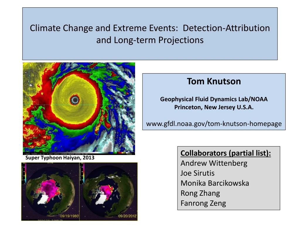
Climate Change and Extreme Events: Detection-Attribution and Long-term Projections. Tom Knutson Geophysical Fluid Dynamics Lab/NOAA Princeton, New Jersey U.S.A. www.gfdl.noaa.gov/tom-knutson-homepage. Collaborators (partial list): Andrew Wittenberg Joe Sirutis Monika Barcikowska

E N D
Climate Change and Extreme Events: Detection-Attribution and Long-term Projections Tom Knutson Geophysical Fluid Dynamics Lab/NOAA Princeton, New Jersey U.S.A. www.gfdl.noaa.gov/tom-knutson-homepage Collaborators (partial list): Andrew Wittenberg Joe Sirutis Monika Barcikowska Rong Zhang Fanrong Zeng Super Typhoon Haiyan, 2013
Talk Outline – Highlights of GFDL Work on Extremes • Hurricanes and Climate Change: • No detectable human influence on hurricanes yet. • Late 21st century projections: increased Category 4-5 hurricane frequency. • Examples of attribution for recent climate extremes • Temperatures (seasonal- or annual-mean warm extremes) • Australia region (2013) – risk increase fully attributable to anthro. forcing • Eastern U.S. (Spring 2012) - risk increased 10x by anthro. + natural forcing • Precipitation (seasonal- or annual-mean extremes) • Northern U.S. region (2013) – risk increased 2-3x by anthro. + natural forcing • Arctic sea ice: 2012 extreme loss – difficult for models to capture • The “global warming hiatus” • CMIP5 models are inconsistent with observations (data-available regions) • lack of observations in Arctic may affect this conclusion for globalmean
IPCC AR5 Summary for Policymakers (Sept. 2013) [Statements related to TCs and climate change] Phenomenon: - Increase in intense tropical cyclone activity Assessment that changes occurred: - Low confidence in long-term (centennial) changes - Virtually certain in North Atlantic since 1970 Assessment of a human contribution to observed changes: - Low confidence - “There is medium confidence that a reduction in aerosol forcing over the North Atlantic has contributed at least in part in the observed increase in tropical cyclone activity since the 1970s in this region.” Likelihood of further changes (late 21st century): - More likely than not (Western North Pacific and N. Atlantic)
TROPICAL CYCLONES SUMMARY ASSESSMENT: Detection and Attribution: It remains uncertain whether past changes in any tropical cyclone activity (frequency, intensity, rainfall, etc.) exceed the variability expected through natural causes, after accounting for changes over time in observing capabilities. Source: WMO Expert Team on Climate Change Impacts on Tropical Cyclones. February 2010
Category 4-5 Tropical Cyclones: 20 yr simulations CMIP5/RCP4.5 Late 21st Century vs. Present Day Storm Category 24% increase in Cat 4-5 frequency globally
Explaining Extreme Events from a Climate Perspective… Regional Surface Temperature anomalies for 2013 Dec.-Feb. 2013 anomalies Mar.-May 2013 anomalies Annual 2013 anomalies Sept.-Nov. 2013 anomalies June-Aug. 2013 anomalies
Surface temperature seasonal- or annual-mean extremes for 2013 Dec.-Feb. 2013 seasonal extremes Mar.-May 2013 seasonal extremes Annual means: 2013 extremes June-Aug. 2013 seasonal extremes Sept.-Nov. 2013 seasonal extremes
Sliding Trend Analysis Australia Region: Annual Temperatures Observed Trends Attributable to External Forcing Non-Detectable Trends Beginning Year of Trend (All Trends Ending in 2013) Attributable Risk Analysis Occurrence Ratio = inf. Ratio = pALL pNAT pALL and pNAT : probabilities of exceeding the threshold in the All Forcing and Natural distributions
Where were the 2012 anomalies ranked 1st, 2nd, 3rdwarmest or coldest? MAM 2012 extremes DJF 2012 extremes Annual 2012 extremes JJA 2012 extremes SON 2012 extremes
An assessment of the extreme March-May 2012 temperatures over the eastern U.S. b) Trend assessment Black Line: HadCRUT4 observations Red Line: CMIP5 All-Forcing ensemble mean Pink: 5th/95th range for CMIP5 All-Forcing ens. Green: 5th/95th range for CMIP5 Control runs Purple: Green/Pink shading overlap oC/100yr Trend start year (all trends ending in 2012) Ratio = pALL = 11 to 12 pCON pALL and pCON : probabilities of exceeding the 2012 or 1991 thresholds in the All Forcing and Control distributions
Annual Mean Precipitation Extremes for 2013 (100 yrs+ of record) mm/day
U.S. Northern Tier region U.S. Northern Tier—ANN: Significant increasing trend; Trend attributable to Anthro. + Natural Annual 2013 Extremes - Precipitation California region California region -- ANN: Non-significant trend Highest 2nd highest Map 3rd highest Legend 3rd lowest 2nd lowest Lowest
Sliding Trend Analysis Observed Trends Attributable to External Forcing U.S. Northern Tier Region – Annual mean Precipitation Non-Detectable Trends Beginning Year of Trend (All Trends Ending in 2013) Attributable Risk Analysis Occurrence Ratio: 2.4 to 3.1 Ratio = pALL pCON pALL and pCON : probabilities of exceeding the 2013 or 2010 thresholds in the All Forcing and Control distributions
Fig. 1 Mar.-May 2013 Extremes - Precipitation U.S. Southern Plains—Mar.-May U.S. Southern Plains region—Mar.-May: Non-significant trend; Data inhomogeneities? June-Aug. 2013 Extremes - Precipitation Eastern U.S. – June-August Eastern U.S. region -- JJA: Non-significant trend from 1900; Detectable trend from 1950 or later; Detection not robust to excluding 2013 Trend attributable to Anthro. + Natural Occurrence Ratio = 1.7 or undefined Highest 2nd highest Map 3rd highest Legend 3rd lowest 2nd lowest Lowest
Arctic Sea Ice Is Decreasing… Source: University of Illinois – The Cryosphere Today
Arctic Sea Ice Extent Anomalies During 2012: An Extreme Year September Arctic Sea Ice Extent Anomaly September Global Mean Temperature Anomaly Source: Rong Zhang and Thomas Knutson, BAMS, 2013.
September 2012: Arctic Sea Ice Extent Anomaly vs. Global SAT Anomaly Source: R. Zhang and T. Knutson, BAMS, 2013.
Global Mean Surface Temperature Anomalies a) CMIP5: All Forcings (Anthro. + Natural) b) CMIP5: Natural forcing only (solar & volcanic) All Forcing: Anthropogenic (well-mixed GHGs, ozone, aerosols, land use change) + Natural Forcing Natural Forcing: Solar variability; volcanic aerosols
Consider the distributions of 15-yr trends from a climate model for the period 1997-2012. • The mean of the model’s distribution is the ensemble mean of the model’s historical run ensemble over the period in question. • The spread about the mean for the model is the distribution of 15-year trends from the model’s control run. Observed Trend Occurrence frequency 15-yr trends [oC/decade]
Consider three distributions of 15-yr trends from three different models for the period 1997-2012. • The mean of each model’s distribution is the ensemble mean of that model’s historical run ensemble over the period in question. • The spread about the mean for each model is the distribution of 15-year trends from the control run of that model. Observed Trend Occurrence frequency 15-yr trends [oC/decade]
Are missing temperature observations in the Arctic causing the hiatus? Source: Realclimate.org (Rahmsdorf, Nov. 13, 2013, after Cowtan and Way, QJRMS, 2014.).
Summary – Highlights of GFDL Work on Extremes • Hurricanes and Climate Change: • No detectable human influence on hurricanes yet. • Late 21st century projections: increased Category 4-5 hurricane frequency. • Examples of attribution for recent climate extremes • Temperatures (seasonal- or annual-mean warm extremes) • Australia region (2013) – risk increase fully attributable to anthro. forcing • Eastern U.S. (Spring 2012) - risk increased 10x by anthro. + natural forcing • Precipitation (seasonal- or annual-mean extremes) • Northern U.S. region (2013) – risk increased 2-3x by anthro. + natural forcing • Arctic sea ice: 2012 extreme loss – difficult for models to capture • The “global warming hiatus” • CMIP5 models are inconsistent with observations (data-available regions) • lack of observations in Arctic may affect this conclusion for globalmean
Extra slides: (for Q&A period)
1901-2010 Surface Temperature Trend Assessment Observed trend (HadCRUT4) CMIP5 All-Forcing ensemble trend CMIP5 All-Forcing vs. Natural-Forcing assessment Attrib. anthro. warming, but > simulated Attrib. & consistent anthro. warming Detectable warming: < simulated No detectable trend Detectable cooling: < simulated Attributable anthropogenic cooling Detectable cooling: > simulated
North Atlantic GFDL HIRAM 50 km grid model TC simulations corr=0.83 red: observations blue: HiRAM ensemble mean shading: model uncertainty East Pacific corr=0.62 GFDL HIRAM 50km grid global model (SST-forced): Simulated vs Observed Tropical Storm Tracks (1981-2005) West Pacific corr=0.52 Source: Zhao, Held, Lin, and Vecchi (J. Climate, 2009
Present-Day Climate Storm Category:
Normalized histogram of maximum winds (1980-2008 Obs. SSTs) Present-Day Climate GFDL dynamical downscaling to 6 km grid model; preliminary results 2013.
St. Deviation of low-freq. (>10 yr) variability: Model vs. Observed* a) CMIP3: 8-model-avg. b) Obs. St. Dev.* (CMIP3) oC 0.8 0.7 0.6 0.5 0.4 0.3 0.2 0.1 0 c. ) CMIP5: 23-model-avg d) Obs. St. Dev.* (CMIP5_23) Notes: Model estimate is from control runs; observed estimate is based on the residual with All-Forcing ensemble mean subtracted. An additional adjustment was made to reduce the systematic error due to the computation method for creating the residual. We let each ensemble member substitute for observations in the computation procedure.