Download
1 / 31
310 likes | 444 Vues
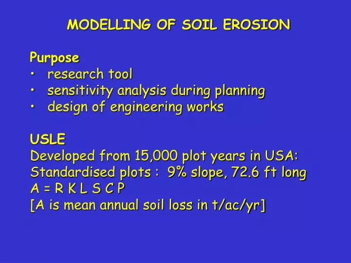
MODELLING OF SOIL EROSION Purpose research tool sensitivity analysis during planning design of engineering works USLE Developed from 15,000 plot years in USA: Standardised plots : 9% slope, 72.6 ft long A = R K L S C P [A is mean annual soil loss in t/ac/yr]. Rainfall

E N D
MODELLING OF SOIL EROSION • Purpose • research tool • sensitivity analysis during planning • design of engineering works • USLE • Developed from 15,000 plot years in USA: • Standardised plots : 9% slope, 72.6 ft long • A = R K L S C P • [A is mean annual soil loss in t/ac/yr]
Rainfall R = rainfall factor = erosivity/100 = kinetic energy x maximum 30 minute intensity (but this parameter is a simplification of what is going on & may not be applicable in some instances) Monthly and annual EI30 are calculated by summation of individual storms.
Definition of a storm: • average intensity must be > 0.25 mm/hr • must be separated by > 2 hrs from last rain (otherwise counted as same storm) • at least one 5 minute with > 25 mm/hr • > 12.5 mm total.
To calculate EI30 from first principles, drop size distribution. v. intensity required. Therefore, equations such as the following have been derived to eliminate need for drop size - assumes relationship between drop size and intensity: logarithmic relationship - reciprocal relationship Note these are per mm of rain. For a whole year sum EI30 for each storm.
Other people have looked for regional equations to find relationships between : • Es & I(t) throughout the storm • Es & R (and sometimes I30) • EsI30 to Rs (and sometimes I30) • R » 0.5 x annual rainfall in tropics [approx.] • where R, the rainfall erosivity index, is the • average yearly total of EI30 / 100 in ft-ton/acre • and rainfall in mm. • See handout for equations for predicting rain erosivity.
More precisely for Kenya: R = 0.29 Ey - 26 [in British units where R is the rainfall erosivity index and Ey is the annual kinetic energy of the raindrops] 1 Another source2 gives (again for Kenya): Ey = 22P - 15795 (in metric units where here P is the annual rainfall amount in mm) 1Soil Cons. in Kenya? 2Soil conservation for agroforestry?
Example (from Morgan, p. 47) Energy per mm of rain calculated from: E = 29.8 - 127.5/I (for Zimbabwe - see above) Maximum 30 minute rainfall = 26.16 + 31.5 = 57.66 Maximum 30 minute intensity = 57.66 x 2 = 115.32 mm h-1 Total kinetic energy = 2277.74 J m-2 [total of column 5] EI30 = 2277.74 x 115.32 = 262669 J m-2 mm h-1 Hudson index of erosivity (KE>25) - energy for rain over 25 mm h-1 = rows 2, 3, 4 & 5 of column 5 = 2264 J m-2 mm h-1
Other factors in USLA Erodibility K = soil erodibility factor (mean annual soil loss per unit of erosivity) defined such that K is erosion rate relative to that from a standard plot 22 m long & 9% slope with no conservation practices. Examples shown overleaf
Length & degree of slope L= slope length factor [relative to loss from 22m] S = slope steepness factor [relative to loss from 9%] L & S factors are usually combined into a LS factor.
One of the earliest equations was due to Zingg (1940): A = C S1.4 L0.6 where A was the average soil loss per unit of AREA , C was a constant, S was land slope (%), L was slope length (ft). Soil loss per unit WIDTH of slope would be A = C S1.4 L1.6
In Wischmeier & Smith (no relation) equation: “LS” = (l0.5/22.13) x (0.065 + 0.045s + 0.0065s²) Note that this factor relates to the soil loss per unit area. For soil loss per unit WIDTH, the exponent would be 1.5.
Cover and management factor C = cover and management factor [relative to bare fallow] e.g. C = 0.8 for maize or tobacco C = 0.01 for well managed tea C = 0.001 for natural rain forest other values in table following To arrive at an annual factor, the variation of crop morphology throughout the year needs to be taken into account. Ground cover such as stubble between the cropping seasons is also allowed for.
Can be divided into three parts : - C-I - for plant canopy cover (for a given % cover, taller crops have a higher C-I) C-II - % of soil surface covered by mulch C-III - root network from previously undisturbed land
In RUSLE, C = PLU . CC . SC . SR where PLU is a previous land use factor, CC is a crop canopy factor, SC is surface or ground cover factor and SR is a surface roughness factor
Practice factor P = practice factor [relative to erosion from field with plant rows up/down slope]. If neither contouring nor strip cropping practised and no other conservation measures, the value is 1.0 e.g. P = 0.4 for strip cropping P = 0.05 to 0.1 for well maintained terraces USLE needs modifying and calibration for use in the tropics. This has been done for some countries such as India, Ethiopia
Example of the effect of ground cover 2% slope at Nyankapa, Nigeria3 Bare fallow was the control Groundnut cover was an intercrop 3Bonsu. 1980. Erosion & cultural practices. In Morgan, 1980. p. 251
SLEMSA (Soil Loss Estimation Model for South Africa) Z = KCX t/ha/yr where: K = soil loss from 30 m plot @ 4% == f(rain energy, soil) C = crop factor = f(energy intercepted) C = 0.3 if 0.2 energy intercepted C = 0.1 if 0.4 energy intercepted C = 0.05 if 0.5 energy intercepted X = topographic factor = f(slope angle, length) = LS of Wischmeier & Smith, approximately
FAO • This a simplified version of the USLE used by the FAO: • A = RKSC (ignores length & management) • designed for large scale mapping of relative potential erosion
Musgrave type erosion Some experiments on unrilled slopes show a rapid increase (over a few metres) of sediment load carried by overland flow to a capacity which remains relatively constant regardless of slope length. The basic equation is: where y is the sediment yield, q the overland flow and s the slope angle Morgan (1980) gives:
Others • Hairsine-Rose model • Rose model [- both complex mathematical models for detachment, entrainment, and deposition] • CREAMS (Chemicals, Runoff, and erosion from agricultural management systems) • EPIC (Erosion Productivity Impact Calculator) • SCUAF (Soil changes under agroforestry) • RUSLE (Revised Universal Soil Loss Equation) - see Hudson, 1995 for summary of changes • WEPP (Water Erosion Prediction Project; theoretical analysis; meant to replace USLE see Chapter 5 in Morgan; also Hudson, 1995 • Stehlík (for Czech Rep. & Slovakia)
Indices of soil erodibility See Table 1 Handout It gives various methods of comparing soil erodibility. Apart from the K value of Wischmeier and Smith, these cannot be used in the USLE directly. They would need to be calibrated and related to K.
Estimates of K from soil properties • A method of estimating K from soil properties is given in Figure 1. • You need estimates of • organic matter content • percentage sand (0.1 to 2 mm) • percentage of silt to very fine sand • soil structure • permeability
Starting with the percentage of silt + v. fine sand, enter the diagram on the left vertical axis. Continue horizontally until you meet the percent sand curves (running from top left to bottom right) and stop when you reach the curve corresponding to the sample's value for sand. Then go vertically until you reach the Organic Matter (OM) group of curves and stop when you reach the sample's OM value. Then go horizontally into the second diagram and stop when you reach the soil structure curves. Proceed downward until you reach the permeability curves and stop when you intersect the curves estimated permeability. Then turn horizontally going left until you reach the vertical axis of K. Read off the value.
The example shown is for a soil having • silt + v. fine sand = 65% • sand = 5% • OM = 2.8% • structure = fine granular • permeability = slow to moderate Where the silt fraction does not exceed 70 percent, the equation is 100 K = 2.1 M1.18 (104) (12 - a) + 3.25 (b - 2) + 2.5 (c - 3) where M = (percent si + vfs) (100-percent c), a = percent organic matter, b = structure code c = permeability class
Nomograph for estimating soil erodibility (K) based on soil properties. From Morgan, p. 54, quoting Wischmeier, Johnson and Cross, 1971.