Download
1 / 60
600 likes | 746 Vues
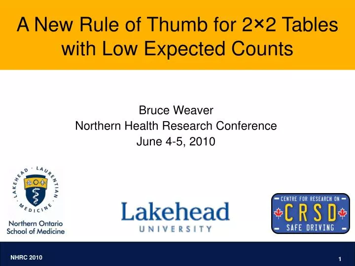
A New Rule of Thumb for 2 × 2 Tables with Low Expected Counts. Bruce Weaver Northern Health Research Conference June 4-5, 2010. Speaker Acceptance & Disclosure. I have no affiliations, sponsorships, honoraria, monetary support or conflict of interest from any commercial source.

E N D
A New Rule of Thumb for 2×2 Tables with Low Expected Counts Bruce Weaver Northern Health Research Conference June 4-5, 2010
Speaker Acceptance & Disclosure • I have no affiliations, sponsorships, honoraria, monetary support or conflict of interest from any commercial source. • However…it is only fair to caution you that this talk has not undergone ethical review of any sort. • Therefore, you listen at your own peril.
A Very Common Problem “One of the commonest problems in statistics is the analysis of a 2×2 contingency table.” Ian Campbell (Statist. Med. 2007; 26:3661–3675)
What’s a contingency table? See the example on the next slide.
Example: A 2×2 Contingency Table What the heck is malocclusion? Counts in the cells
Normal Occlusion vs. Malocclusion Class IOcclusion. Normal occlusion. The upper teeth bite slightly ahead of the lowers. Class II Malocclusion. Upper teeth bite greatly ahead of the lower teeth—i.e., overbite. Class IIIMalocclusion. Upper front teeth bite behind the lower teeth—i.e., under-bite.
What statistical test can I use to analyze the data in my contingency table? It depends.
The Most Commonly Used Test • The most common statistical test for contingency tables is Pearson’s chi-squared test of association. Karl Pearson Greek letter chi Observed count Sum Expected count
But you can’t always use Pearson’s • It is well known (to those who know it well)* that Pearson’s chi-square is an approximate test A typical chi-square distribution • The sampling distribution of the test statistic (under a true null hypothesis) is approximated by a chi-square distribution with df = (r-1)(c-1) • The approximation becomes poor when the expected counts (assuming H0 is true) are too low * Robert Rankin, author of The Hollow Chocolate Bunnies of the Apocalypse.
How low is too low for expected counts? It depends. Again, it depends! This guy is starting to get on my nerves.
A Rule of Thumb for 2×2 Tables • A common rule of thumb for when it’s OK to analyze a 2×2 table with Pearson’s chi-squared test of association says: • All expected counts should be 5 or greater • If any expected counts are < 5, another test should be used • The most frequently recommended alternative test under point 2 above is Fisher’s exact test (aka the Fisher-Irwin test)
Some History • The standard rule of thumb for 2×2 tables dates back to Cochran (1952, 1954), or even earlier • But, the minimum expected count of 5 appears to have been an arbitrary choice (probably by Fisher) • Cochran (1952) suggested that it may need to be modified when new evidence became available. • Computations by Ian Campbell (2007) have provided some new & relevant evidence.
The Role of Research Design • Three distinct research designs can give rise to 2×2 tables • Barnard (1947) classified them as follows: G.A. Barnard • Model I: • Model II: • Model III: Both row & column totals fixed in advance Row totals fixed, column totals free to vary Both row & column totals free to vary
Campbell on Model I “Here, there is no dispute that the Fisher–Irwin test … should be used.” “This last research design is rarely used and will not be discussed in detail.” Ian Campbell (Statist. Med. 2007; 26:3661–3675, emphasis added)
Review of Models II and III • Model II • Sometimes called the 2×2 comparative trial • Row totals fixed, column totals free to vary • E.g., researcher fixes group sizes for Treatment & Control groups, or for Males & Females • Model III • Also called a cross-sectional study • Both row & column totals are free to vary • Only the total N is fixed
So what did Campbell do? “Computer-intensive techniques were used … to compare seven two-sided tests of two-by-two tables in terms of their Type I errors.” Ian Campbell (Statist. Med. 2007; 26:3661–3675
Let’s try that again… • Null hypothesis was always true – i.e., there was no association between the row & column variables • Therefore, statistically significant results were Type I errors • For values of N ranging from 4-80, Campbell computed the maximum probability of Type I error(with alpha set to .05) • He also examined all possible values of π The proportion of subjects (in the population) having the binary characteristic(s) of interest—e.g., the proportion of males, or the proportion of smokers, etc
The statistical tests of interest • Campbell examined 7 different statistical tests • I will focus on only 2 of those tests today: • Pearson’s chi-square • The ‘N-1’ chi-square
The ‘N-1’ chi-square Pearson’s chi-square (shortcut for 2×2 tables only) The ‘N-1’ chi-square (for 2×2 tables only)
Whence the ‘N-1’ chi-square? • First derived by E.S. Pearson (1947) • Egon Sharpe Pearson, son of Karl • Derived again by Kendall & Stuart (1967) • Richardson (1994) asserted that it is “the appropriate chi-square statistic to use in analysing all 2×2 contingency tables” (p. 116, emphasis added) • Campbell summarizes the theoretical argument for preferring the N-1 chi-square on his website: • www.iancampbell.co.uk/twobytwo/n-1_theory.htm
Campbell’s Procedure • Campbell computed the maximum Type I error probability for: • N ranging from 4 to 80 • Over all values of π • For minimum expected count = 0, 1, 3, and 5 • He did all of that using both: • Pearson’s chi-squared test of association • The N-1 chi-squared test • Compared the actual Type I error rate to the nominal alpha • All of the above done for Models II and III separately
An Ideal Test • For an ideal test, the actual proportion of Type I errors is equal to the nominal alpha level • E.g., if you set alpha at .05, Type I errors occur 5% of the time (when the null hypothesis is true)
A Conservative Test • A test is if the actual Type I error rate is lower than the nominal alpha • Conservative tests have low power – they don’t reject H0 as often as they should (i.e., too many Type II errors)
A Liberal Test • A test is if the actual Type I error rate is higher than the nominal alpha • Liberal tests reject H0 too easily, or too frequently (i.e., too many Type I errors)
Cochran’s Criterion for Acceptable Test Performance • With discrete data (like counts) and small sample sizes, the actual Type I error rate is generally not exactly equal to the nominal alpha • Cochran (1942) suggested allowing a 20% error in the actual Type I error rate—e.g., for nominal alpha = .05, an actual Type I error rate between .04 and .06 is acceptable • Cochran’s criterion is admittedly arbitrary, but other authors have generally followed it (or a similar criterion) – and Campbell (2007) uses it.
Figure 2A: Pearson chi-square (Model II) with minimum E = 0, 1, 3, and 5 Minimum value of E Maximum over all values of π .05 ± 20% (from Cochran) For Model II, Pearson’s chi-squared test meets Cochran’s criterion only if the minimum E≥ 5 (the blue line).
Figure 2B: N-1 chi-square (Model II)with minimum E = 0, 1, 3, and 5 Minimum value of E For Model II, the N-1 chi-squared test meets Cochran’s criterion quite well for expected counts as low as 1.
Figure 4A: Pearson chi-square (Model III) with minimum E = 0, 1, 3, and 5 Minimum value of E For Model III, Pearson’s chi-squared test meets Cochran’s criterion fairly well for E as low as 3.
Figure 4B: N-1 chi-square (Model III) with minimum E = 0, 1, 3, and 5 Minimum value of E For Model III, the N-1 chi-squared test meets Cochran’s criterion very well for expected counts as low as 1.
Campbell’s New Rule of Thumb for 2×2 Tables • For Model I – row & column totals both fixed • Use the two-sided Fisher Exact Test(as computed by SPSS) • Aka the Fisher-Irwin Test “by Irwin’s rule” • For Models II and III – comparative trials & cross-sectional • If all E≥ 1, use the ‘N − 1’ chi-squared test • Otherwise, use the Fisher–Irwin Test by Irwin’s rule
Increased Power • Campbell’s new rule of thumb “extends the use of the chi-squared test to smaller samples … with a resultant increase in the power to detect real differences.” (Campbell, 2007, p. 3674, emphasis added) And as everyone knows, the more power, the better! Tim “the Stats-Man” Taylor & Al
Campbell’s Online Calculator http://www.iancampbell.co.uk/twobytwo/calculator.htm
Computing the N-1 chi-square with SPSS • I have written 2 SPSS syntax files to compute the N-1 chi-square • Ian Campbell provides a link to them beside his online calculator A link to my two SPSS syntax files
Questions? Yeah, I have a question. Did you have to include that picture? Severe Malocclusion
References Barnard GA. Significance tests for 2×2 tables. Biometrika 1947; 34:123–138. Campbell I. Chi-squared and Fisher–Irwin tests of two-by-two tables with small sample recommendations. Statist. Med. 2007; 26:3661–3675. [See also: http://www.iancampbell.co.uk/twobytwo/twobytwo.htm] Cochran WG. The χ2 test of goodness of fit. Annals of Mathematical Statistics 1952; 25:315–345. Cochran WG. Some methods for strengthening the common χ2 tests. Biometrics 1954; 10:417–451. Kempthorne O. In dispraise of the exact test: reactions. Journal of Statistical Planning and Inference 1979;3:199–213. Kendall MG, Stuart A. The advanced theory of statistics, Vol. 2, 2nd Ed. London: Griffin, 1967. Pearson ES. The choice of statistical tests illustrated on the interpretation of data classed in a 2×2 table. Biometrika 1947; 34:139–167. Rankin R. The Hollow Chocolate Bunnies of the Apocalypse. Gollancz (August 1, 2003). Richardson JTE. The analysis of 2x1 and 2x2 contingency tables: A historical review. Statistical Methods in Medical Research 1994; 3:107-133.
Etymology of rule of thumb • However, there is no solid evidence to support that claim • http://www.phrases.org.uk/meanings/rule-of-thumb.html • http://www.canlaw.com/rights/thumbrul.htm • http://womenshistory.about.com/od/mythsofwomenshistory/a/rule_of_thumb.htm • http://www.straightdope.com/columns/read/2550/does-rule-of-thumb-refer-to-an-old-law-permitting-wife-beating • Some have claimed that the expression rule of thumb derives an old legal ruling in England that allowed men to beat their wives with a stick, provided it was no thicker than their thumb
An Important Topic "The importance of the topic cannot be stressed too heavily." "2×2 contingency tables are the most elemental structures leading to ideas of association.... The comparison of two binomial parameters runs through all sciences." Dr. Oscar Kempthorne (J Stat Planning and Inf 1979;3:199–213, emphasis added)
Oscar Kempthorne (1919-2000) • Farm boy from Cornwall who became a Cambridge-trained statistician • In 1941, he joined Rothamsted Experiment Station, where he met Ronald Fisher and Frank Yates • Strongly influenced by Fisher—e.g., areas of interest were experimental design, genetic statistics, and statistical inference Kempthorne & Fisher
J.O. Irwin (1898-1982) “J. O. Irwin was a soft spoken kind soul who took a tremendous interest in his students and their achievements.... He was a lovable absent-minded kind of professor who smoked more matches than he did tobacco in his ever-present pipe while he was deeply involved in thinking about other important matters.” Major Greenwood “His old boss Pearson and his new boss R. A. Fisher were bitter enemies but Irwin's conciliatory nature allowed him to remain on good terms with both men.” From http://en.wikipedia.org/wiki/Joseph_Oscar_Irwin
A Variation on the Rule • A variation on that rule of thumb says that: • All expected counts should be 10 or greater. • If any expected counts are less than 10, but greater than or equal to 5, Yates' Correction for continuity should be applied. (However, the use of Yates' correction is controversial, and is not recommended by all authors). • If any expected counts are less than 5, then some other test should be used. • Again, the most frequently recommended alternative test under point 3 has been Fisher’s exact test.
Figure 1: Maximum Type I error probability for comparative trials (Model II) Maximum over all values of π Far too liberal if we impose no restrictions on minimum value of E Cochran’s range: ± 20% of .05 Arguably too conservative for smaller values of N
Figure 3: Maximum Type I error probability for cross-sectional studies (Model III) Too liberal if we impose no restrictions on minimum value of E Again, the FET is too conservative
Pearson’s chi-square • O = observed count • E = expected count (assuming a true null hypothesis) • Σ = Greek letter sigma & means to sum across all cells General formula for contingency tables of any size
I don’t remember what expected counts are—can you explain that? Of course. See the next slide.
Example: A 5×2 Table E = row total × column total / grand total
How low is too low for expected counts? It depends. If I had a dollar for every time I heard a statistician say that, I’d be rich.
It depends on the table dimensions • For contingency tables larger than 2×2, the chi-square approximation is pretty good if: • Many people do not know this, and mistakenly assume that all expected counts must be 5 or more for tables of any size “…no more than 20% of the expected counts are less than 5 and all individual expected counts are 1 or greater." (Yates, Moore & McCabe, 1999, p. 734)