Download
1 / 41
720 likes | 2.9k Vues
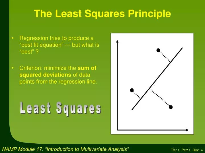
Regression tries to produce a “best fit equation” --- but what is “best” ? Criterion: minimize the sum of squared deviations of data points from the regression line. The Least Squares Principle. Least Squares. (Sum of squares about mean of Y) (Sum of squares about regression line).

E N D
Regression tries to produce a “best fit equation” --- but what is “best” ? Criterion: minimize the sum of squared deviations of data points from the regression line. The Least Squares Principle Least Squares
(Sum of squares about mean of Y) (Sum of squares about regression line) How Good is the Regression (Part 1) ? How well does the regression equation represent our original data? The proportion (percentage) of the of the variance in y that is explained by the regression equation is denoted by the symbol R2. R2=
High R2 - good explanation Low R2 - poor explanation Explained Variability - illustration
Remember you used a sample from the population of potential data points to determine your regression equation. e.g. one value every 15 minutes, 1-2 weeks of operating data A different sample would give you a different equation with different coefficients bi As illustrated on the next slide, the sample can greatly affect the regression equation… How Good is the Regression (Part 2) ? How well would this regression equation predict NEW data points?
Sampling variability of Regression Coefficients - illustration Sample 2: y = a’’x + b’’ + e Sample 1: y = a’x + b’ + e
Confidence limits (x%) are upper and lower bounds which have an x% probability of enclosing the true population value of a given variable Often shown as bars above and below a predicted data point: Confidence Limits
Data used for regression are usually normalised to have mean zero and variance one. Otherwise the calculations would be dominated (biased) by variables having: numerically large values large variance This means that the MVA software never sees the original data, just the normalised version Normalisation of Data
Each variable is represented by a variance bar and its mean (centre). Normalisation of Data - illustration Mean-centred only Variance- centred only Raw data Normalised
Data Requirements Normalised data Errors normally distributed with mean zero Independent variables uncorrelated Implications if Requirements Not Met Larger confidence limits around regression coefficients (bi) Poorer prediction on new data Requirements for Regression
Principal Component Analysis (PCA) X’s only Projection to Latent Structures (PLS) a.k.a. “Partial Least Squares” X’s and Y’s Multivariate Analysis Now we are ready to start talking about multivariate analysis (MVA) itself. There are two main types of MVA: Xx Can be same dataset, i.e., you can do PCA on the whole thing (X’s and Y’s together) X Y Let’s start with PCA. Note that the European food example at the beginning was PCA, because all the food types were treated as equivalent.
The purpose of PCA is to project a data space with a large number of correlated dimensions (variables) into a second data space with a much smaller number of independent (orthogonal) dimensions. This is justified scientifically because of Ockham’s Razor. Deep down, Nature IS simple. Often the lower dimenional space corresponds more closely to what is actually happening at a physical level. The challenge is interpreting the MVA results in a scientifically valid way. Purpose of PCA Reminder… “Ockham’s Razor”
Advantages of PCA Among the advantages of PCA: • Uncorrelated variables lend themselves to traditional statistical analysis • Lower-dimensional space easier to work with • New dimensions often represent more clearly the underlying structure of the set of variables (our friend Ockham) -1 +1 Reminder… “Latent Attributes”
Find a component (dimension vector) which explains as much x-variation as possible Find a second component which: is orthogonal to (uncorrelated with) the first explains as much as possible of the remaining x-variation Process continues until researcher satisfied or increase in explanation is judged minimal How PCA works (Concept) PCA is a step-wise process. This is how it works conceptually:
How PCA Works (Math) This is how PCA works mathematically: • Consider an (n x k) data matrix X(n observations, k variables) • PCS models this as(assuming normalized data): X = T * P’ + E • whereTis the scores of each observation on the new componentsPis the loadings of the original variables on the new componentsE residual matrix, containing the noise Like linear regression only using matrices
. . . . . . . . . . . . How PCA Works (Visually) The way PCA works visually is by projecting the multidimensional data cloud onto the “hyperplane” defined by the first two components. The image below shows this in 3-D, for ease of understanding, but in reality there can be dozens or even hundreds of dimensions: X3 X2 Data cloud (in red) is projected onto plane defined by first 2 components X1 3 original variables
Number of Components Components are simply the new axes which are created to explain the most variance with the least dimensions. The PCA methodology ensures that components are extracted in decreasing order of explained variance. In other words, the first component always explains the most variance, the second component explains the next most variance, and so forth: 1 2 3 4 5 6 . . . Eventually, the higher-level components represent mainly noise. This is a good thing, and in fact one of the reasons we use PCA in the first place. Because noise is relegated to the higher-level components, it is absent from the first few components. This is because all components are orthogonal to each other, which means that they are statistically independent or uncorrelated.
Eigenvalues of a matrix A : Mathematically defined by (A - I) = 0 Useful as an “importance measure” for variables The Eigenvalue Criterion • There are two ways to determine when to stop creating new components: • Eigenvalue criterion • Scree test • The first of these uses the following mathematical definition: • Usually, components with eigenvalues less than one are discarded, since they have less explanatory power than the original variables did in the first place.
The second method is a simple graphical technique: Plot eigenvalues vs. number of components Extract components up to the point where the plot “levels off” Right-hand tail of the curve is “scree” (like lower part of a rocky slope) 8 7 6 5 4 3 2 1 Eigenvalue 1 2 3 4 5 6 Component # The Inflection Point Criterion (Scree Test)
Look at strength and direction of loadings Look for clusters of variables which may be physically related or have a common origin e.g., In papermaking, strength properties such as tear, burst, breaking length in the paper are all related to the length and bonding propensity of the initial fibres. Interpretation of the PCA Components As with any type of MVA, the most difficult part of PCA is interpreting the components. The software is 100% mathematical, and gives the same outputs whether the data relates to diesel fuel composition or last night’s horse racing results. It is up to the engineer to make sense of the outputs. Generally, you have to:
PCA vs. PLS What is the difference between PCA and PLS? PLS is the multivariate version of regression. It uses two different PCA models, one for the X’s and one for the Y’s, and finds the links between the two. Mathematically, the difference is as follows: In PCA, we are maximising the variance that is explained by the model. In PLS, we are maximising the covariance. Xx X Y
PLS finds a set of orthogonal components that : maximize the level of explanation of both X and Y provide a predictive equation for Y in terms of the X’s This is done by: fitting a set of components to X (as in PCA) similarly fitting a set of components to Y reconciling the two sets of components so as to maximize explanation of X and Y How PLS works (Concept) PLS is also a step-wise process. This is how it works conceptually:
How PLS works (Math) This is how PLS works mathematically: • X = TP’ + Eouter relation for X(like PCA) • Y = UQ’ + Fouter relation for Y(like PCA) • uh = bhthinner relation for componentsh = 1,…,(# of components) • Weighting factors w are used to make sure dimensions are orthogonal
PLS – the “Inner Relation” The way PLS works visually is by “tweeking” the two PCA models (X and Y) until their covariance is optimised. It is this “tweeking” that led to the name partial least-squares. All 3 are solved simultaneously via numerical methods
Interpretation of the PLS Components Interpretation of the PLS results has all the difficulties of PCA, plus one other one: making sense of the individual components in both X and Y space. In other words, for the results to make sense, the first component in X must be related somehow to the first component in Y. Note that throughout this course, the words “cause” and “effect” are absent. MVA determines correlations ONLY. The only exception is when a proper design-of-experiment has been used. Here is an example of a false correlation: the seed in your birdfeeder remains full all winter, then suddenly disappears in the spring. You conclude that the warm weather made the seeds disintegrate…
Types of MVA Outputs MVA software generates two types of outputs: results, and diagnostics. We have already seen the Score plot and Loadings plot in the food example. Some others are shown on the next few slides. • Results • Score Plots • Loadings Plots • Diagnostics • Plot of Residuals • Observed vs. Predicted • …(many more) Already seen…
Residuals • Also called “Distance to Model” (DModX) • Contains all the noise • Definition: DModX = ( eik2 / D.F.)1/2 • Used to identify moderate outliers • Extreme outliers visible on Score Plot (next slide) Original observations
“Distance to Model” . eik i=observationk=variable
Observed vs. Predicted This graph plots the Y values predicted by the model, against the original Y values. A perfect model would only have points along the diagonal line. IDEAL MODEL
Here is a list of some of the main challenges you will encounter when doing MVA. You have been warned! Difficulty interpreting the plots (“like reading tea leaves”) Data pre-processing Control loops can disguise real correlations Discrete vs. averaged vs. interpolated data Determining lags to account for flowsheet residence times Time increment issues e.g., second-by-second values, or daily averages? Some typical sensitivity variables for the application of MVA to real process data are shown on the next page… MVA Challenges
End of Tier 1 Congratulations! Assuming that you have done all the reading, this is the end of Tier 1. No doubt much of this information seems confusing, but things will become more clear when we look at real-life examples in Tier 2. All that is left is to complete the short quiz that follows…
Tier 1 Quiz • Question 1: • Looking at one or two variables at a time is not recommended, because often variables are correlated. What does this mean exactly? • These variables tend to increase and decrease in unison. • These variables are probably measuring the same thing, however indirectly. • These variables reveal a common, deeper variable that is probably unmeasured. • These variables are not statistically independent. • All of the above.
Tier 1 Quiz • Question 2: • What is the difference between “information” and “knowledge”? • Information is in a computer or on a piece of paper, while knowledge is inside a person’s head. • Only scientists have “true” knowledge. • Information is mathematical, while knowledge is not. • Information includes relationships between variables, but without regard for the underlying scientific causes. • Knowledge can only be acquired through experience.
Tier 1 Quiz • Question 3: • Why does MVA never reveal cause-and-effect, unless a designed experiment is used? • Cause-and-effect can only be determined in a laboratory. • Designed experiments eliminate error. • MVA without a designed experiment is only inductive, whereas a cause-and-effect relationship requires deduction. • Only effects are measurable. • Scientists design experiments to work perfectly the first time.
Tier 1 Quiz • Question 4: • What is the biggest disadvantage to using a “black-box” model instead of one based on first principles? • There are no unit operations. • The model is only as good as the data used to create it. • Chemical reactions and thermodynamic data are not used. • A black-box model can never take into account the entire flowsheet. • MVA models are linear only.
Tier 1 Quiz • Question 5: • What does a confidence interval tell you? • How widely your data are spread out around a regression line. • The range within which a certain percentage of sample values can be expected to lie. • The area within which your regression line should fall. • The level of believability of the results of a specific analysis. • The number of times you should repeat your analysis to be sure of your results
Tier 1 Quiz • Question 6: • When your data were being recorded, one of the mill sensors was malfunctioning and giving you wildly inaccurate readings. What are the implications likely to be for statistical analysis? • More square and cross-product terms in the model you fit to the data. • Higher mean values than would normally be expected. • Higher variance values for the variables associated with the malfunctioning sensor. • Different selection of variables to include in the analysis. • Bigger residual term in your model.
Tier 1 Quiz • Question 7: • Why does reducing the number of dimensions (more variables to fewer components) make sense from a scientific point of view? • The new components might correspond to underlying physical phenomena that can’t be measured directly. • Fewer dimensions are easier to view on a graph or computer output. • Ockham’s Razor limits scientists to less than five dimensions. • The real world is limited to just three dimensions. • All of the above.
Tier 1 Quiz • Question 8: • If two points on a score plot are almost touching, does that mean that these two observations are nearly identical? • Yes, because they lie in the same position within the same quadrant. • No, because of experimental error. • Yes, because they have virtually the same effect on the MVA model. • No, because the score plot is only a projection. • Answers (a) and (c).
Tier 1 Quiz • Question 9: • Looking at the food example, what countries appear to be correlated with high consumption of olive oil? • Italy and Spain, and to a lesser degree Portugal and Austria. • Italy and Spain only. • Just Italy. • Ireland and Italy. • All the countries except Sweden, Denmark and England.
Tier 1 Quiz • Question 10: • Why does error get relegated to higher-order components when doing PCA? • Because Ockham’s Razor says it will. • Because the real world has only three dimensions. • Because noise is false information. • Because MVA is able to correct for poor data. • Because noise is uncorrelated to the other variables.