Download
1 / 19
190 likes | 344 Vues
SOFTWARE METRICS USING CONSTRUCTIVE COST MODEL. By K Gopal Reddy. Introduction . Metrics in software are of two types .direct and indirect . Function points as indirect metrics . Function points are used to measure the effort of the project Cost estimation model .

E N D
SOFTWARE METRICS USING CONSTRUCTIVE COST MODEL By K Gopal Reddy
Introduction • Metrics in software are of two types .direct and indirect . • Function points as indirect metrics . • Function points are used to measure the effort of the project • Cost estimation model
What is cost estimation model ? • Why use cost estimation ? • How are they calculated ?
Cost estimation model is used to calculate the effort and schedule of a project . • Cost estimation models give easy ways for risk mitigation and prepare plan for building the project . • They are calculated using cost drivers . • What are cost drivers ? • Cost drivers are critical features that have a direct impact on the project.
CONSTRUCTIVE COST MODEL • It was developed by Barry W Boehm in the year 1981. • It is an algorithmic cost model. • It is based on size of the project. • The size of the project may vary depending upon the function points .
COCOMO MODELS • Basic cocomo • used for relatively smaller projects . • team size is considered to be small. • Cost drivers depend upon size of the projects . • Effort E = a * (KDSI) b * EAF Where KDSI is number of thousands of delivered source instructions a and b are constants, may vary depending on size of the project . • schedule S= c * (E) d where E is the Effort and c, d are constants. • EAF is called Effort Adjustment Factor which is 1 for basic cocomo , this value may vary from 1 to 15.
Classes of software projects • Organic mode projects • Used for relatively smaller teams. • Project is developed in familiar environment. • There is a proper interaction among the team members and they coordinate their work. • Bohem observed E=2.4(KDSI)1.05 E in person-months. • And S=2.5(E)0.38.
Semidetached mode projects • It lies between organic mode and embedded mode in terms of team size. • It consists of experienced and inexperienced staff. • Team members are unfamiliar with the system under development. • Bohem observed E=3(KDSI)1.12 E in person-months. • S.35=2.5(E)0And
Embedded mode projects • The project environment is complex. • Team members are highly skilled. • Team members are familiar with the system under development. • Bohem observed E=3.6(KDSI)1.20 E in person-months. • And S=2.5(E)0.32.
Intermediate COCOMO • It is used for medium sized projects. • The cost drivers are intermediate to basic and advanced cocomo. • Cost drivers depend upon product reliability, database size, execution and storage. • Team size is medium. • Advanced COCOMO • It is used for large sized projects. • The cost drivers depend upon requirements, analysis, design, testing and maintenance. • Team size is large.
LIMITATIONS OF COCOMO • COCOMO is used to estimate the cost and schedule of the project, starting from the design phase and till the end of integration phase. For the remaining phases a separate estimation model should be used. • COCOMO is not a perfect realistic model. Assumptions made at the beginning may vary as time progresses in developing the project. • When need arises to revise the cost of the project. A new estimate may show over budget or under budget for the project. This may lead to a partial development of the system, excluding certain requirements. • COCOMO assumes that the requirements are constant throughout the development of the project; any changes in the requirements are not accommodated for calculation of cost of the project. • There is not much difference between basic and intermediate COCOMO, except during the maintenance and development of the software project. • COCOMO is not suitable for non-sequential ,rapid development, reengineering ,reuse cases models.
COST ESTIMATION ACCURACY • The cost estimation may vary due to changes in the requirements, staff size, and environment in which the software is being developed. • The calculation for cost estimation accuracy is given as follows • Absolute error= (Epred - Eactual) • Percentage error= (Epred - Eactual)/Eactual • Relative error= 1/n ∑ (Epred - Eactual)/Eactual • The above results give a more accurate estimation of costs for future projects.The cost estimation model now becomes more realistic .
COCOMO II • COCOMOII was developed in 1995 • It could overcome the limitations of calculating the costs for non-sequential, rapid development, reengineering and reuse models of software. • It has 3 modules • Application composition: - good for projects with GUI interface for rapid development of project. • Early design: - Prepare a rough picture of what is to be designed. Done before the architecture is designed. • Post architecture: - Prepared after the architecture has been designed.
COCOMO II calculation • In COCOMO II the constant value b is replaced by 5 scale factors. • Effort (E) is calculated as follows E = a * (KDSI) sf * π (EM) • Where a is constant, sf is scaling factor, EM is Effort Multiplier (7 for Early design, 17 for Post architecture).
COCOMO II USES • Helps in making decisions based on business and financial calculations of the project. • Establishes the cost and schedule of the project under development, this provides a plan for the project. • Provides a more reliable cost and schedule, hence the risk mitigation is easy to accomplish. • It overcomes the problem of reengineering and reuse of software modules. • Develops a process at each level . Hence takes care of the capability maturity model.
CONCLUSION • Constructive Cost Model was developed by Barry W Boehm, is the most common and widely used cost estimation models for most software projects. • The effort and schedule calculated by the model is based on two things, historical information and experience. Thus the reliability on cocomo has been increased. • The website provided by NASA on cocomo, provides a cocomo calculator with cost drivers for a complex project. Cost drivers directly have an impact on the development of the project.
References • [1] Farshad Faghih,” Software Effort and Schedule Estimation”, http://www2.enel.ucalgary.ca/People/Smith/619.94/prev689/1997.94/reports/farshad.htm • [2]IAN SOMMERVILLE,” Software Engineering”, published by addision wesley, pg 514- 521. • [3]Seth Bowen, Samuel Lee, Lance Titchkosky,”Software cost estimation”, http://www.computing.dcu.ie/~renaat/ca421/BLTCostEst.ppt • [4]Barry Boehm, “Cost Estimation With COCOMO II”,http://sunset.usc.edu/classes/cs577a_2002/lectures/19/ec19.pdf • [5]Center for Systems and Software engineering, “COCOMO II”, http://sunset.usc.edu/csse/research/COCOMOII/cocomo_main.html.

![UNIT-25 COCOMO [CONSTRUCTIVE COST MODEL]](https://cdn4.slideserve.com/672242/slide1-dt.jpg)