Download
1 / 38
680 likes | 1.38k Vues
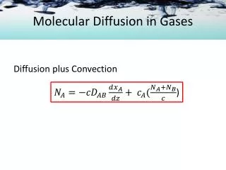
Principles of Mass Transfer Molecular Diffusion in Liquids. Where solute A is diffusing and solvent B is stagnant or nondiffusing. Example: Dilute solution of propionic Acid (A) in water (B) being contact with toluene. EXAMPLE 6.3-1. An ethanol ( A )-water ( B ) solution in the form of

E N D
Principles of Mass Transfer Molecular Diffusion in Liquids
Where solute A is diffusing and solvent B is stagnant or nondiffusing. Example: Dilute solution of propionic Acid (A) in water (B) being contact with toluene.
EXAMPLE 6.3-1 An ethanol (A)-water (B) solution in the form of a stagnant film 2.0 mm thick at 293 K is in constant at one surface with an organic solvent in which ethanol is soluble and water is insoluble. Hence, NB = 0. At point 1 the concentration of ethanol is 16.8 wt % and the solution density is ρ1 = 972.8 kg/m3. At point 2 the concentration of ethanol is 6.8 wt % and ρ2 = 988.1 kg/m3. The diffusivity of ethanol is 0.740 x 10⁻⁹ m2/s. Calculate the steady-state flux NA.
Solution The diffusivity of ethanol is 0.740 x 10⁻⁹ m2/s. The molecular weights of A and B are MA= 46.05 and MB=18.02. for a wt % of 6.8, the mole fraction of ethanol (A) is as follows when using 100 kg solution: Then XB2 = 1-0.0277 = 0.9723. Calculating XA1 = 0.0732 and XB1 = 1-0.0732 = 0.9268. To calculate the molecular weight M2 at point 2,
Similarly, M1 = 20.07. From Eq. (6.3-2), To calculate XBM from Eq. (6.3-4), we can use the linear mean since XB1 and XB2 are close to each other: Substituting into Eq. (6.303) and solving,
Principles of Mass Transfer Molecular Diffusion in Solids
EXAMPLE 6.5-1 The gas hydrogen at 17 °C and 0.010 atm partial pressure is diffusing through a membrane of vulcanized neoprene rubber 0.5 mm thick. The pressure of H2 on the other side of the neoprene is zero. Calculate the steady-state flux, assuming that the only resistance to diffusion is in the membrane. The solubility S of H2 gas in neoprene at 17 °C is 0.0151 m3 (at STP of 0 °C and 1 atm)/m3 solid.atm and the diffusivity DAB is 1.03 x 10⁻¹⁰ m2/s at 17 °C.
Solution A sketch showing the concentration is shown in Fig. 6.5-1. The equilibrium concentration cA1 at the inside surface of the rubber is, from Eq. (6.5-5), Since pA2 at the other side is 0, cA2 = 0. Substituting into Eq. (6.5-2) and solving, FIGURE 6.5-1 concentrations for Example 6.5-1
EXAMPLE 6.5-2 A polyethylene film 0.00015 m (0.15 mm) thick is being considered for use in packaging a pharmaceutical product at 30 °C. If the partial pressure of O2 outside the package is 0.21 atm and inside it is 0.01 atm, calculate the diffusion flux of O2 at steady state. Use permeability data from Table 6.5-1. Assume that the resistances to diffusion outside the film and inside are negligible compared to the resistance of the film.
Solution From Table 6.5-1, PM = 4.17 (10-12) m3 solute (STP)/(s.m2.atm/m). Substituting into Eq. (6.5-8)
EXAMPLE 6.5-3 A sintered solid of silica 2.0 mm thick is porous, with a void friction εof 0.30 and a tortuosityτ of 4.0. The pores are filled with water at 298 K. At one face the concentration of KCl held at 0.10 g mol/liter, and fresh water flow rapidly past the other face. Neglecting any other resistance but that in the porous solid, calculate the diffusion of KCl at steady state.
Solution The diffusivity of KCL in water from Table 6.3-1 is DAB= 1.87 x 10⁻⁹ m2/s. Also, cA1 = 0.10/1000 = 1.0 x 10⁻⁴ g mol/m3, and cA2 = 0. Substituting into Eq. (6.5-13),
Molecular Diffusion in Biological Solutions and Gels
Diffusion of Biological Solutes in Liquids • Important: The diffusion of solute molecules (macromolecules) • Food processing: drying of fruit juice, coffee, tea, water, volatile flavor • Fermentation process: diffuse through microorganisms like nutrient, sugar, oxygen • Table 6.4-1 shows Diffusion Coefficient for Dilute Biological Solutes in Aqueous Solution.
Prediction of Diffusivities for Biological Solutes • Small solutes in aqueous solution with molecular weight less than 1000 or solute molar less than about 0.500 m3/kgmol • For larger solutes, an approximation the Stokes-Einstein equation can be used
Prediction of Diffusivities for Biological Solutes For a molecular weight above 1000
EXAMPLE 6.4-1 Predict the diffusivity of bovine serum albumin at 298 K in water as a dilute solution using the modified Polson equation and compare with the experimental value in Table 6.4-1.
Solution The molecular weight of bovine serum albumin (A) from Table 6.4-1 is MA= 67500 kg/kg mol. The viscosity of water at 25 °C is 0.8937 x 10⁻³ Pa.s at T = 298 K. Substituting into Eq. (6.4-1), This value is 11% higher than the experimental value of 6.81 x 10⁻¹¹ m2/s
Diffusion in Biological Gels • Gel can be looked as semisolid materials which are porous. • Example: agarose, agar, gelatin. • The pores or open spaces in the gel structure are filled with water. • The rates of diffusion of small solutes in the gels are somewhat less than in aqueous solution. • A few typical values of diffusivities of some solutes in various gel are given in Table 6.4.2.
EXAMPLE 6.4-2 A tube or bridge of a gel solution of 1.05 wt % agar in water at 278 K is 0.04 m long and connects two agitated solutions of urea in water. The urea concentration in the first solution is 0.2 g mol urea per liter solution and is 0 in the other. Calculate the flux of urea in kg mol/s.m2 at steady state.
Solution From Table 6.4-2 for the solute urea at 278 K, DAB = 0.727 x 10⁻⁹ m2/s. For urea diffusing through stagnant water in the gel, Eq. (6.3-3) can be used. However, since the value of xA1 is less than about 0.01, the solution is quite dilute and xBM 1.00. Hence Eq. (6.3- 5) can be used. The concentrations are cA1= 0.20/1000 = 0.0002 g mol/cm3 = 0.20 kg mol/m3 and cA2= 0. Substituting into Eq. (6.3-5),