Download
1 / 52
560 likes | 997 Vues
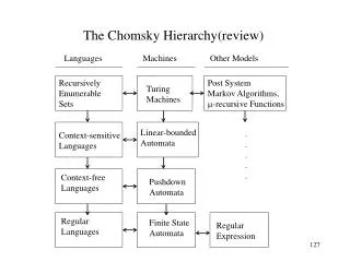
The Chomsky Hierarchy and Beyond. Chapter 24. Is There Anything In Between PDAs and Turing Machines?. PDAs aren’t powerful enough. Turing machines lack even a decision procedure for the acceptance problem. Linear Bounded Automata.

E N D
The Chomsky Hierarchy and Beyond Chapter 24
Is There Anything In Between PDAs and Turing Machines? • PDAs aren’t powerful enough. • Turing machines lack even a decision procedure for the acceptance problem.
Linear Bounded Automata • A linear bounded automaton is an NDTM the length of whose tape is equal to |w| + 2. • Example: AnBnCn = {anbncn : n 0} • qaabbccqqqqqqqqq
Linear Bounded Automata • A language is context sensitive iff there exists an LBA that accepts it. • Note: It is not known whether, for every nondeterministic LBA there exists an equivalent deterministic one.
The Membership Question for LBAs Let L = {<B, w> : LBA B accepts w}. Is L in D? … qabbaq … q0 How many distinct configurations of B exist?
The Membership Question for LBAs Let L = {<B, w> : LBA B accepts w}. Is L in D? … qabbaq … q0 How many distinct configurations of B exist? MaxConfigs = |K| ||(|w|+2) (|w| + 2)
The Membership Question for LBAs Theorem: L = {<B, w> : LBA B accepts w} is in D. Proof: If B runs for more than MaxConfig steps, it is in a loop and it is not going to halt. M is an NDTM that decides L: M(<B, w>) = 1. Simulate all paths of B on w for MaxConfig steps or until B halts, whichever comes first. 2. If any path accepted, accept. Else reject. Since, from each configuration of B there are a finite number of branches and each branch is of finite length, M will be able to try all branches of B in a finite number of steps. M will accept the string <B, w> if any path of B accepts and it will reject the string <B, w> if every path of B on w either rejects or loops.
Grammars, Context-Sensitive Languages, and LBAs CS Language L Grammar Accepts LBA
Context-Sensitive Grammars and Languages A context-sensitive grammarG = (V, , R, S) is an unrestricted grammar in which R satisfies the following constraints: ● The left-hand side of every rule contains at least one nonterminal symbol. ● No length-reducing rules, with one exception: Consider: S aSb S /* length reducing
Context-Sensitive Grammars and Languages A context-sensitive grammarG = (V, , R, S) is an unrestricted grammar in which R satisfies the following constraints: ● The left-hand side of every rule contains at least one nonterminal symbol. ● No length-reducing rules, with one exception: ● R may contain the rule S. If it does, then S does not occur on the right hand side of any rule.
Context-Sensitive Grammars and Languages Example of a grammar that is not context-sensitive: SaSb S An equivalent, context-sensitive grammar:
Context-Sensitive Grammars and Languages Example of a grammar that is not context-sensitive: SaSb S An equivalent, context-sensitive grammar: S ST TaTb Tab
AnBnCn AnBnCn SaBSc S /* Not a CS rule BaaB Bcbc Bbbb
Equal Numbers of a’s, b’s, and c’s {w {a, b, c}* : #a(w) = #b(w) = #c(w)} SABCS S ABBA BCCB ACCA BAAB CAAC CBBC Aa Bb Cc
WW WW = {ww : w {a, b}*} ST# /* Generate the wall exactly once. TaTa /* Generate wCwR. TbTb TC CCP /* Generate a pusher P PaaaPa /* Push one character to the right to get ready to jump. PabbPa PbaaPb PbbbPb Pa# #a /* Hop a character over the wall. Pb# #b C#
The Membership Question for Context-Sensitive Grammars Let L = {<G, w> : csg G generates string w}. Is L in D? Example: SaBSc SaBc BaaB Bcbc Bbbb S aBScaBaBSccaaBBScc …
L = {<G, w> : CSG G generates string w} is in D. Proof: We construct an NDTM M to decide D. M will explore all derivations that G can produce starting with S. Eventually one of the following things must happen on every derivation path: ● G will generate w. ● G will generate a string to which no rules can be applied. ● G will keep generating strings of the same length. Since there are a finite number of strings of a given length, G must eventually generate the same one twice. The path can be terminated since it is not getting any closer to generating w. ● G will generate a string s that is longer than w. Since G has only a finite number of choices at each derivation step and since each path that is generated must eventually halt, the Turing machine M that explores all derivation paths will eventually halt. If at least one path generates w, M will accept. If no path generates w, M will reject.
Context-Sensitive Languages and Linear Bounded Automata Theorem: The set of languages that can be generated by a context-sensitive grammar is identical to the class that can be accepted by an LBA. Proof: (sketch) ● Given a CSG G, build a two-track LBA B such that L(B) = L(G). On input w, B keeps w on the first track. On the second track, it nondeterministically constructs all derivations of G. As soon as any derivation becomes longer than |w|, stop. ● From any LBA B, construct a CSG that simulates B.
Languages and Machines SD D Context-sensitive Context-free DCF Regular FSMs DPDAs NDPDAs LBAs Turing machines
Context-Sensitive Languages vs. D Theorem: The CS languages are a proper subset of D. Proof: We divide the proof into two parts: ● Every CS language is in D: Every CS language L is accepted by some LBA B. The Turing machine that performs a bounded simulation of B decides L. ● There exists at least one language that is in D but that is not context-sensitive: It is not easy to do this by actually exhibiting such a language. But we can use diagonalization to show that one exists.
Using Diagonalization Create an encoding for context-sensitive grammars: x00ax00a;x00x01;x01bx01b;x01b EnumG is the lexicographic enumeration of all encodings of CSGs with = {a, b}. Enuma,b is the lexicographic enumeration of {a, b}*. Because {<G, w> : CSG G generates string w}, is in D, there exists a TM that can compute the values in this table as they are needed.
Diagonalization, Continued Define LD = {stringi : stringiL(Gi)}. LD is: ● Recursive because it is decided by the following Turing machine M: M(x) = 1. Find x in the list Enuma,b. Let its index be i. 2. Lookup cell (i, i) in the table. 3. If the value is 0, x is not in L(Gi) so x is in L. Accept. 4. If the value is 1, x is in L(Gi) so x is not in L. Reject. ● Not context-sensitive because it differs, in the case of at least one string, from every language in the table and so is not generated by any context-sensitive grammar.
Context-Sensitive vs Context-Free • Theorem: The context-free languages are a proper subset of the • context-sensitive languages. • Proof: We divide the proof into two parts: • ● We know one language, AnBnCn, that is context-sensitive but • not context-free. • ● If L is a context-free language then there exists some context-free • grammar G = (V, , R, S) that generates it: • ● Convert G to G in Chomsky normal form • ● G generates L – {}. • ● G has no length-reducing rules, so is a CSG. • ● If L, add to G the rules S and SS. • ● G is still a context-sensitive grammar and it generates L. • ● So L is a context-sensitive language.
Closure Properties The context-sensitive languages are closed under: ● Union ● Concatenation ● Kleene star ● Intersection ● Complement
Closure Under Union • Theorem: The CSLs are closed under union. • Proof: By construction of a CSG G such that L(G) = L(G1) L(G2): • If L1 and L2 are CSLs, then there exist CSGs: • G1 = (V1, 1, R1, S1) and • G2 = (V2, 2, R2, S2) such that L1 = L(G1) and L2 = L(G2). • Rename the nonterminals of G1 and G2 so that they are disjoint • and neither includes the symbol S. • G will contain all the rules of both G1 and G2. Add to G a new start symbol, S, and two new rules: • SS1 and SS2. • So G = (V1V2 {S}, 12, • R1R2 {SS1, SS2}, S).
Closure Under Concatenation Theorem: The CSLs are closed under concatenation. Proof: By construction of a CSG G such that L(G) = L(G1) L(G2): If L1 and L2 are CSLs, then there exist CSGs G1 = (V1, 1, R1, S1) and G2 = (V2, 2, R2, S2) such that L1 = L(G1) and L2 = L(G2). Let G contain all the rules of G1 and G2. Then add a new start symbol, S, and one new rule, SS1S2. Problem: S S1S2 a aA a a a The subtrees may interact.
Nonterminal Normal Form A CSG G = (V, , R, S) is in nonterminal normal form iff all rules in R are of one of the following two forms: ● c, where is an element of (V - ) and c, ● , where both and are elements of (V - )+. A aBBc is not in nonterminal normal form. aAB BB is not in nonterminal normal form.
Nonterminal Normal Form Theorem: Given a CSG G, there exists an equivalent nonterminal normal form grammar G such that L(G) = L(G). Proof: The proof is by construction. converttononterminal(G: CSG) = 1. Initially, let G = G. 2. For each terminal symbol c in , create a new nonterminal symbol Tc. Add to RG the rule Tcc. 3. Modify each of the original rules so that every occurrence of a terminal symbol c is replaced by the nonterminal symbol Tc. 4. Return G. AA aBBc becomes AA TaBBTc Ta a Tc c aAB BB becomes TaAB BB
Closure Under Concatenation S S1S2 a aA a a a Now the subtrees will be: S S1S2 a aATa a a We prevent them from interacting by standardizing apart the nonterminals.
Concatenation, Continued To build a grammar G such that L(G) = L(G1) L(G2), we do the following: 1. Convert both G1 and G2 to nonterminal normal form. 2. If necessary, rename the nonterminals of G1 and G2 so that the two sets are disjoint and so that neither includes the symbol S. 3. Let G = (V1V2 {S}, 12, R1R2 {SS1S2}, S).
Decision Procedures The membership problem is decidable, although no efficient procedure is known. Other questions are not: ● Is L empty? ● Is the intersection of two CSLs empty? ● Is L = *? ● Are two CSLs equal?
Attribute, Feature and Unification Grammars The idea: constrain rule firing by: ● defining features that can be passed up/down in parse trees, and ● describing feature-value constraints that must be satisfied before the rules can be applied.
AnBnCn G will exploit one feature, size. G = ({S, A, B, C, a, b, c},{a, b, c}, R, S), where: R = { SABC (size(A) = size(B) = size(C)) Aa (size(A) 1) AA2a (size(A) size(A2) + 1) Bb (size(B) 1) BB2b (size(B) size(B2) + 1) Cc (size(C) 1) CC2c (size(C) size(C2) + 1) }. Applying G bottom up: aaabbbccc
A Unification Grammar for Subject/Verb Agreement * The bear like chocolate. The culprit is the rule SNPVP. Replace NP and VP by: [ CATEGORY NP [ CATEGORY VP PERSON THIRDPERSON THIRD NUMBER SINGULAR] NUMBER SINGULAR] Replace atomic terminal symbols like bear, with: [ CATEGORY N LEX bear PERSON THIRD NUMBER SINGULAR]
A Unification Grammar for Subject/Verb Agreement Replace SNPVP with: [ CATEGORY S] [ CATEGORY NP [ CATEGORY VP NUMBERx1NUMBERx1 PERSONx2 ] PERSONx2 ] So an NP and a VP can be combined to form an S iff they have matching values for their NUMBER and PERSON features.
Lindenmayer Systems An L-system G is a triple (, R, ), where: ● is an alphabet, which may contain a subset C of constants, to which no rules will apply, ● R is a set of rules, ● (the start sequence) is an element of +. Each rule in R is of the form: A, where: ● A. A is the symbol that is to be rewritten by the rule. ●, *. and describe context that must be present in order for the rule to fire. If they are equal to , no context is checked. ●*. is the string that will replace A when the rule fires.
Rules Fire in Parallel Using a standard grammar: Given: A S a B B a B S a B B a B S a Ca B a etc. Using an L-system: Given: A S a B B a B F a Ha Ha a
A Lindenmayer System Interpreter • L-system-interpret(G: L-system) = • 1. Set working-string to . • 2. Do forever: • 2.1 Output working-string. • 2.2 new-working-string = . • 2.3 For each character c in working-string do: • If possible, choose a rule r whose left-hand side • matches c and where c’s neighbors (in • working-string) satisfy any context constraints • included in r. • If a rule r was found, concatenate its right-hand side • to the right end of new-working-string. • If none was found, concatenate c to the right end of • new-working-string. • 2.4 working-string = new-working-string.
An Example Let G be the L-system defined as follows: = {I, M}. = I. R = {IM, MM I }. The sequence of strings generated by G begins: 0. I 1. M 2. M I 3. M I M 4. M I M M I 5. M I M M I M I M 6. M I M M I M I M M I M M I
Fibonacci’s Rabbits Assume: ● It takes one time step for each rabbit to reach maturity and mate. ● The gestation period of rabbits is one time step. ● We begin with one pair of (immature) rabbits. The Fibonacci sequence: Fibonacci0 = 1. Fibonacci1 = 1. For n > 1, Fibonaccin = Fibonnacin-1 + Fibonnacin-2. The L-system model: ● Each I corresponds to one immature pair of rabbits. ● Each M corresponds to one mature pair. ● Each string is the concatenation of its immediately preceding string (the survivors) with the string that preceded it two steps back (the breeders).
Fibonacci’s Rabbits 0. I 1. M 2. M I 3. M I M 4. M I M M I 5. M I M M I M I M 6. M I M M I M I M M I M M I
Sierpinski Triangle Let G be the L-system defined as follows: = {A, B, +, -}. = A. R = { AB – A – B, BA + B + A }. Notice that + and – are constants. The sequence of strings generated by G begins: 1. A 2. B – A – B 3. A + B + A – B – A – B – A + B + A 4. B – A – B + A + B + A + B – A – B – A + B + A – B – A – B – A + B + A – B – A – B + A + B + A + B – A – B
Interpreting Strings as Drawing Programs ● Choose a line length k. ● Attach meanings to the symbols in as follows: ● A and B mean move forward, drawing a line of length k. ● + means turn to the left 60. ● – means turn to the right 60. Strings 3, 4, 8, and 10 then correspond to turtle programs that can draw the following sequence of figures (scaling k appropriately):
Modelling Plant Growth Let G be the L-system defined as follows: = {F, +, –, [, ]}. = F. R = { FF [ – F ] F [ + F ] [ F ] }. The sequence of strings generated by G begins: 1. F 2. F [ – F ] F [ + F ] [ F ] 3. F [ – F ] F [ + F ] [ F ] [ – F [ – F ] F [ + F ] [ F ] ] F [ – F ] F [ + F ] [ F ] [ + F [ – F ] F [ + F ] [ F ] ] [ F [ – F ] F [ + F ] [ F ] ]
Interpreting Strings as Drawing Programs We can interpret these strings as turtle programs by choosing a line length k and then attaching meanings to the symbols in as follows: ● F means move forward, drawing a line of length k. ● + means turn to the left 36. ● – means turn to the right 36. ● [ means push the current pen position and direction onto the stack. ● ] means pop the top pen position/direction off the stack, lift up the pen, move it to the position that is now on the top of the stack, put it back down, and set its direction to the one on the top of the stack. 3. F [ – F ] F [ + F ] [ F ] [ – F [ – F ] F [ + F ] [ F ] ] F [ – F ] F [ + F ] [ F ] [ + F [ – F ] F [ + F ] [ F ] ] [ F [ – F ] F [ + F ] [ F ] ]
Sierpinski Triangles, Again Let G be the L-system defined as follows: = {, }. = . R = { ( | ) () , ( | ) ( | ) , () () , () ( | ) , ( | ) () , ( | ) ( | ) , () () , () ( | ) }.