Download
1 / 40
460 likes | 648 Vues
Visibility Graphs and Cell Decomposition. By David Johnson. Shakey the Robot. Built at SRI Late 1960’s For robotics, the equivalent of Xerox PARC’s Alto computer Alto – mouse, GUI, network, laser printer, WYSIWYG, multiplayer computer game

E N D
Visibility GraphsandCell Decomposition By David Johnson
Shakey the Robot • Built at SRI • Late 1960’s • For robotics, the equivalent of Xerox PARC’s Alto computer • Alto – mouse, GUI, network, laser printer, WYSIWYG, multiplayer computer game • Shakey – mobile, wireless, path-planning, Hough transform, camera vision, English commands, logical reasoning
Shakey path planning • Represent the world as a hierarchical grid • Full • Partially-full • Empty • Unknown • Compute nodes at corners of objects • Find shortest path through nodes – A*
Shakey used two good ideas • A* • Putting sub-goals on corners of vertices • This has been generalized into the idea of visibility graphs.
Visibility Graphs • Define undirected graph VG(N,L) • V = all vertices of obstacles • N = V union (Start,Goal) • L = all links (ni,nj) such that there is no overlap with any obstacle. Polygon edge doesn’t count as overlapping.
Reusing Visibility Graphs • Add new visibility edges for new start/goal points • The rest is unchanged • Creates a roadmap to follow
Visibility Graph in Motion Planning • Start with geometry of robot and obstacles, R and O • Compute the Minkowski difference of O – R • Compute visibility graph in C-space • Search graph for shortest path
Computing the Visibility Graph • Brute force • Check every possible edge against all polygon edges
Computing the Visibility Graph • Brute force • Check every possible edge against all polygon edges
Computing the Visibility Graph • Brute force • Check every possible edge against all polygon edges
Computing the Visibility Graph • Brute force • Check every possible edge against all polygon edges
Computing the Visibility Graph • Brute force • Check every possible edge against all polygon edges
Computing the Visibility Graph • Brute force • Check every possible edge against all polygon edges
Computing the Visibility Graph • Brute force • Check every possible edge against all polygon edges
Computing the Visibility Graph • Brute force • Check every possible edge against all polygon edges
Computing the Visibility Graph • Brute force • Check every possible edge against all polygon edges
Special Cases • Do include polygon edges that don’t intersect other polygons • Don’t include edges that cross the interior of any polygon • Minkowski difference of original obstacles may overlap
Reduced VG tangent segments • Eliminate concave obstacle vertices • (line would continue on into obstacle)
Generalized tangency point
Shortest path passes through none of the vertices Three-dimensional Space • Original paper split up long line segments so there were lots of vertices to work with • Computing the shortest collision-free path in a general polyhedral space is NP-hard • Exponential in dimension
Roadmaps and Coverage • Visibility Graphs make a roadmap through space • Roadmaps not so good for coverage of free space • What kind of robot needs to cover C-free?
Roadmaps and Coverage • Roadmaps not so good for coverage of free space • Vacuum robots • Minesweeper robots • Farming robots • Try to characterize the free space
Cell Decomposition • Representation of the free space using simple regions called cells A cell
Exact Cell Decomposition • Exact Cell Decomposition • Decompose all free space into cells Exact Approximate
Coverage • Cell decomposition can be used to achieve coverage • Path that passes an end effector over all points in a free space • Cell has simple structure • Cell can be covered with simple motions • Coverage is achieved by walking through the cells
Cell Decomposition • Two cells are adjacent if they share a common boundary • Adjacency graph: • Node correspond to a cell • Edge connects nodes of adjacent cells
Path Planning • Path Planning in two steps: • Planner determines cells that contain the start and goal • Planner searches for a path within adjacency graph
c14 c7 c4 c5 c8 c2 c15 c11 c1 c10 c13 c3 c9 c6 c12 Trapezoidal Decomposition • Two-dimensional cells that are shaped like trapezoids(plus special case triangles)
c14 c7 c4 c5 c8 c2 c15 c11 c1 c10 c1 c13 c3 c9 c6 c12 Adjacency Graph
c14 c7 c4 c5 c8 c2 c15 c11 c1 c10 c1 c3 c13 c3 c9 c6 c12 Adjacency Graph
c14 c7 c4 c5 c8 c2 c15 c11 c1 c10 c1 c2 c3 c13 c3 c9 c6 c12 Adjacency Graph
c14 c7 c4 c5 c8 c2 c15 c11 c1 c10 c7 c8 c9 c11 c4 c5 c2 c1 c6 c3 c13 c3 c9 c6 c12 c14 c15 c13 c12 c10 Adjacency Graph
Path Planner • Search in adjacency graph for path from start cell to goal cell • First, find nodes in path
c14 c7 c4 c5 c8 c2 c15 c11 c1 c10 c7 c8 c9 c11 c4 c5 c2 c1 c6 c3 c13 c3 c9 c6 c12 c14 c15 c13 c12 c10 Adjacency Graph
Creating a Path • Trapezoid is a convex set • Any two points on the boundary of a trapezoidal cell can be connected by a straight line segment that does not intersect any obstacle • Path is constructed by connecting midpoint of adjacency edges
c14 c7 c4 c5 c8 c2 c15 c11 c1 c10 c7 c8 c9 c11 c4 c5 c2 c1 c6 c3 c13 c3 c9 c6 c12 c14 c15 c13 c12 c10 Adjacency Graph
c14 c7 c4 c5 c8 c2 c15 c11 c1 c10 c7 c8 c9 c11 c4 c5 c2 c1 c6 c3 c13 c3 c9 c6 c12 c14 c15 c13 c12 c10 What if goal were here?
c14 c7 c4 c5 c8 c2 c15 c11 c1 c10 c13 c3 c9 c6 c12 Trapezoidal Decomposition • Shoot rays up and down from each vertex until they enter a polygon • Naïve approach O(n2) (n vertices times n edges)
Other Exact Decompositions • Triangular cell • Optimal triangulation is NP-hard (exponential in vertices)