Assembly Line Balancing

1. Assembly Line Balancing Jaime Joo MBA 530 – Section 1 Brigham Young University

2. Outline • What is Assembly Line Balancing? • How can Assembly Line Balancing benefit your operations? • Classic approach to ALB • Let’s practice! • ALB in the real world • Conclusions

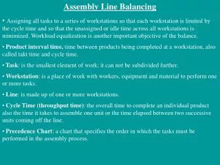
3. What is Assembly Line Balancing (ALB)? ALB is the procedure to assign tasks to workstations so that: • Precedence relationship is complied with • No workstation takes more than the cycle time to complete • Operational idle time is minimized

4. How can Assembly Line Balancing benefit your operations? A balanced line: • Promotes one piece flow • Avoids excessive work load in some stages (overburden) • Minimizes wastes (over-processing, inventory, waiting, rework, transportation, motion) • Reduces variation

5. Unbalanced Line !?  Zzz Zzz 10 sec 40 sec! 20 sec 15 sec Overproduction! Generates waste Undesirable waiting

6. Balanced Line     25 sec 25 sec 20 sec 15 sec • Promotes one piece flow • Avoids overburden • Minimizes wastes • Reduces variation

7. Line Balancing prerequisites Prior to balancing a line we must: • Determine the required workstation cycle time (or TAKT time), matching the pace of the manufacturing process to customer demand • Standardize the process

8. Classic approach to ALB Also known as SALBP* (Simple Assembly Line Balancing Problem), the classic approach to ALB is an heuristic process to optimize assembly lines simplifying the problem to a basic level of complexity *Dubbed SALBP by Becker and Scholl (2004)

9. Example The next table shows the tasks performed in a production line. Our goal is to combine them into workstations. The assembly line operates 8 hours per day and the expected customer demand is 1000 units per day. Balance the line and calculate the efficiency and theoretical minimum number of workstations.

10. Example (cont.)

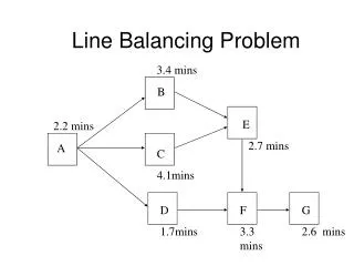
11. Example (cont.) • Step 1: Draw a precedence diagram according to the given sequential relationship 20 sec 11 sec D 18 sec B H 12 sec 13 sec E 15 sec 9 sec A J K 13 sec 17 sec F 15 sec I C 13 sec G

12. Example (cont.) • Step 2: Determine Takt time or Workstation Cycle Time C=Production time per day / Customer demand (or output per day) C= 28800 sec (8 hours) / 1000 units = 28.8 • Step 3: Determine the theoretical number of workstations required N= Total Task Time / Takt time N= 156 / 28.8 = 5.42 (~6 workstations)

13. Example (cont.) • Step 4: Define your assignment rules. For this example our primary rule will be “number of following tasks” and the secondary rule will be “longest operation time”

14. Example (cont.) • Step 5: Assign tasks to workstations following the assignment rules and meeting precedence and cycle time requirements To form Workstation 1: 11 sec 13 sec B Following tasks: 5 A Lot: 15>11! 15 sec C Following tasks: 5 WS1: A+C=28 sec Cycle Time met!

15. Example (cont.) • Forming Workstation 2: 20 sec B+D>Cycle time! D 11 sec 13 sec B 12 sec E LOT:_F&G>E A 15 sec 13 sec C F WS2: Operation time=24 sec (<C) 13 sec G Arbitrarily choose F

16. Example (cont.) • Following the same criteria we achieve our balancing with 7 workstations

17. Example (cont.) • Step 6: Calculate Efficiency • Efficiency= Total Task Time / (Actual number of workstations * Takt Time) • Efficiency= 156 / (7*28.8) = 77% How to interpret this efficiency? Is this the best efficiency achievable?

18. Let’s Practice • We have found a new market for our product. This market is less demanding so we have decided not to include a particular feature, specifically the feature added by task I. As a consequence, task time in F drops to 5 seconds and task time in G drops to 8 seconds. Balance the line according to the other conditions.

19. Let’s practice (cont.)

20. Let’s practice (cont.) • Let’s take some time to solve this new problem. This time we will calculate keeping the primary and secondary rules as in the original problem.

21. Let’s practice (solution) • Precedence diagram 20 sec 11 sec D 18 sec B H 12 sec 13 sec E 15 sec 9 sec A I* J* 5 sec F 15 sec C 8 sec *Previously J & K respectively G

22. Let’s practice (solution) • Takt time C = 28,800 sec / 1000 units = 28.8 • Theoretical number of workstations N = 126/28.8 = 4.38 (~5 workstations) • Primary rule: number of following tasks • Secondary rule: longest operation time

23. Let’s practice (solution) • Following the rules and observing cycle time and precedence we obtain:

24. Let’s practice (solution) • Efficiency = 126/(6*28.8) = 73% Challenge: Is this the best efficiency achievable? Try to solve with LOT as the primary rule and you will obtain a 5 workstations balance, increasing efficiency to 87%

25. ALB in the real world The simple ALB problem approach is limited by some constraints: • Balance on existing and operating lines • Workstations have spatial constraints • Some workstations cannot be eliminated • Need to smooth workload among workstations • Multiple operators per workstation • Different paces among operators, different lead times within the same workstation

26. ALB in the real world (cont.) • Operator spatial constraints • Different workstation imposed working positions • More than one task to be performed in what should be the space for one task • Multiple Products • Coping with different products, some operations are needed for some products but not for others • Some products can introduce “peak times” in some workstations • Different task times performed in different shifts • Particularly when introducing new employees or workers with some degree of incapacity

27. Conclusion • Simply Assembly Line Balancing is a valid method to optimize assembly lines. However, many variables found in real operating lines increase the complexity of the problem. More complex algorithms have been developed to solve the difficult task of balancing large scale industrial lines. Some of them are commercially available in software.

28. References • F. Robert Jacobs & Richard B. Chase “Operations and Supply Management, The Core” McGraw-Hill/Irwin First Edition • Emanuel Falkenauer “Line Balancing in the real world” Optimal Design • Paul Swift. http://www.beyondlean.com/line-balancing.html