Download
1 / 26
260 likes | 452 Vues
Readings: K&F: 9.1, 9.2, 9.3, 9.4. Junction Trees 2. Graphical Models – 10708 Carlos Guestrin Carnegie Mellon University October 22 nd , 2008. What if I want to compute P(X i |x 0 ,x n+1 ) for each i?. X 0. X 2. X 1. X 3. X 4. X 5. Compute:. Variable elimination for each i?.

E N D
Readings: K&F: 9.1, 9.2, 9.3, 9.4 Junction Trees 2 Graphical Models – 10708 Carlos Guestrin Carnegie Mellon University October 22nd, 2008 10-708 – Carlos Guestrin 2006-2008
What if I want to compute P(Xi|x0,xn+1) for each i? X0 X2 X1 X3 X4 X5 Compute: Variable elimination for each i? Variable elimination for every i, what’s the complexity? 10-708 – Carlos Guestrin 2006-2008
Reusing computation X0 X2 X1 X3 X4 X5 Compute: 10-708 – Carlos Guestrin 2006-2008
Cluster graph CD C D I DIG G S GSI L J GJSL JSL H HGJ • Cluster graph: For set of factors F • Undirected graph • Each node i associated with a cluster Ci • Family preserving: for each factor fj2F, 9 node i such that scope[fi] ÍCi • Each edge i – j is associated with a separator Sij = CiÇCj 10-708 – Carlos Guestrin 2006-2008
Cluster graph for VE CD DIG GSI GJSL JSL HGJ • VE generates cluster tree! • One clique for each factor used/generated • Edge i – j, if fi used to generate fj • “Message” from i to j generated when marginalizing a variable from fi • Tree because factors only used once • Proposition: • “Message” dij from i to j • Scope[dij] ÍSij 10-708 – Carlos Guestrin 2006-2008
Running intersection property CD DIG GSI GJSL JSL HGJ • Running intersection property (RIP) • Cluster tree satisfies RIP if whenever X2Ci and X2Cj then X is in every cluster in the (unique) path from Ci to Cj • Theorem: • Cluster tree generated by VE satisfies RIP 10-708 – Carlos Guestrin 2006-2008
Constructing a clique tree from VE • Select elimination order • Connect factors that would be generated if you run VE with order • Simplify! • Eliminate factor that is subset of neighbor 10-708 – Carlos Guestrin 2006-2008
Find clique tree from chordal graph Coherence Difficulty Intelligence Grade SAT Letter Job Happy • Triangulate moralized graph to obtain chordal graph • Find maximal cliques • NP-complete in general • Easy for chordal graphs • Max-cardinality search • Maximum spanning tree finds clique tree satisfying RIP!!! • Generate weighted graph over cliques • Edge weights (i,j) is separator size – |CiÇCj| 10-708 – Carlos Guestrin 2006-2008
Clique tree & Independencies CD DIG GSI GJSL JSL HGJ • Clique tree (or Junction tree) • A cluster tree that satisfies the RIP • Theorem: • Given some BN with structure G and factors F • For a clique tree T for F consider Ci – Cj with separator Sij: • X – any set of vars in Ci side of the tree • Y – any set of vars in Ci side of the tree • Then, (X Y | Sij) in BN • Furthermore, I(T) Í I(G) 10-708 – Carlos Guestrin 2006-2008
Variable elimination in a clique tree 1 C1: CD C2: DIG C3: GSI C4: GJSL C5: HGJ C D I G S L J H • Clique tree for a BN • Each CPT assigned to a clique • Initial potential 0(Ci) is product of CPTs 10-708 – Carlos Guestrin 2006-2008
Variable elimination in a clique tree 2 C1: CD C2: DIG C3: GSI C4: GJSL C5: HGJ • VE in clique tree to compute P(Xi) • Pick a root (any node containing Xi) • Send messages recursively from leaves to root • Multiply incoming messages with initial potential • Marginalize vars that are not in separator • Clique ready if received messages from all neighbors 10-708 – Carlos Guestrin 2006-2008
Belief from message • Theorem: When clique Ci is ready • Received messages from all neighbors • Belief i(Ci) is product of initial factor with messages: 10-708 – Carlos Guestrin 2006-2008
Choice of root Root: node 5 Root: node 3 • Message does not depend on root!!! “Cache” computation: Obtain belief for all roots in linear time!! 10-708 – Carlos Guestrin 2006-2008
Shafer-Shenoy Algorithm (a.k.a. VE in clique tree for all roots) • Clique Ciready to transmit to neighbor Cj if received messages from all neighbors but j • Leaves are always ready to transmit • While 9Ci ready to transmit to Cj • Send message i! j • Complexity: Linear in # cliques • One message sent each direction in each edge • Corollary: At convergence • Every clique has correct belief C2 C3 C1 C4 C5 C6 C7 10-708 – Carlos Guestrin 2006-2008
Calibrated Clique tree • Initially, neighboring nodes don’t agree on “distribution” over separators • Calibrated clique tree: • At convergence, tree is calibrated • Neighboring nodes agree on distribution over separator 10-708 – Carlos Guestrin 2006-2008
Answering queries with clique trees • Query within clique • Incremental updates – Observing evidence Z=z • Multiply some clique by indicator 1(Z=z) • Query outside clique • Use variable elimination! 10-708 – Carlos Guestrin 2006-2008
Introducing message passing with division C1: CD C2: SE C3: GDS C4: GJS • Variable elimination (message passing with multiplication) • message: • belief: • Message passing with division: • message: • belief update: 10-708 – Carlos Guestrin 2006
Factor division • Let X and Y be disjoint set of variables • Consider two factors: 1(X,Y) and 2(Y) • Factor =1/2 • 0/0=0 10-708 – Carlos Guestrin 2006
Lauritzen-Spiegelhalter Algorithm (a.k.a. belief propagation) C1: CD C2: SE C3: GDS C4: GJS Simplified description see reading for details • Separator potentials ij • one per edge (same both directions) • holds “last message” • initialized to 1 • Message i!j • what does i think the separator potential should be? • i!j • update belief for j: • pushing j to what i thinks about separator • replace separator potential: 10-708 – Carlos Guestrin 2006
Convergence of Lauritzen-Spiegelhalter Algorithm C2 C3 C1 C4 C5 C6 C7 • Complexity: Linear in # cliques • for the “right” schedule over edges (leaves to root, then root to leaves) • Corollary: At convergence, every clique has correct belief 10-708 – Carlos Guestrin 2006-2008
VE versus BP in clique trees • VE messages (the one that multiplies) • BP messages (the one that divides) 10-708 – Carlos Guestrin 2006-2008
Clique tree invariant • Clique tree potential: • Product of clique potentials divided by separators potentials • Clique tree invariant: • P(X) = T (X) 10-708 – Carlos Guestrin 2006-2008
Belief propagation and clique tree invariant • Theorem: Invariant is maintained by BP algorithm! • BP reparameterizes clique potentials and separator potentials • At convergence, potentials and messages are marginal distributions 10-708 – Carlos Guestrin 2006-2008
Subtree correctness • Informed message from i to j, if all messages into i (other than from j) are informed • Recursive definition (leaves always send informed messages) • Informed subtree: • All incoming messages informed • Theorem: • Potential of connected informed subtree T’ is marginal over scope[T’] • Corollary: • At convergence, clique tree is calibrated • i = P(scope[i]) • ij = P(scope[ij]) 10-708 – Carlos Guestrin 2006-2008
Clique trees versus VE • Clique tree advantages • Multi-query settings • Incremental updates • Pre-computation makes complexity explicit • Clique tree disadvantages • Space requirements – no factors are “deleted” • Slower for single query • Local structure in factors may be lost when they are multiplied together into initial clique potential 10-708 – Carlos Guestrin 2006-2008
Clique tree summary • Solve marginal queries for all variables in only twice the cost of query for one variable • Cliques correspond to maximal cliques in induced graph • Two message passing approaches • VE (the one that multiplies messages) • BP (the one that divides by old message) • Clique tree invariant • Clique tree potential is always the same • We are only reparameterizing clique potentials • Constructing clique tree for a BN • from elimination order • from triangulated (chordal) graph • Running time (only) exponential in size of largest clique • Solve exactly problems with thousands (or millions, or more) of variables, and cliques with tens of nodes (or less) 10-708 – Carlos Guestrin 2006-2008