Download
1 / 30
320 likes | 463 Vues
An Introduction to Bioconductor. Bethany Wolf Statistical Computing I April 9, 2014. Overview. Background on Bioconductor project Installation and Packages in Bioconductor An example: working with microarray meta-data. Bioconductor.

E N D
An Introduction to Bioconductor Bethany Wolf Statistical Computing I April 9, 2014
Overview • Background on Bioconductor project • Installation and Packages in Bioconductor • An example: working with microarray meta-data
Bioconductor • Biological experiments continually generate more data and larger datasets • Analysis of large datasets is nearly impossible without statistics and bioinformatics • Research groups often re-write the same software with slightly different purposes • Bioconductor includes a set of open-source/open-development tools that are employable in a broad number of biomedical research areas
Bioconductor Project • The Bioconductor project started in 2001 • Goal: make it easier to conduct reproducible consistent analysis of data from new high-throughput biological technologies • Core maintainers of the Bioconductor website located at Fred Hutchinson Cancer Research Center • Updated version released biannually coinciding with the release of R • Like R, there are contributed software packages
Goals of the Bioconductor Project • Provide access to statistical and graphical tools for analysis of high-dimensional biological data • micro-array analysis • analysis of high-throughput • Include comprehensive documentation describing and providing examples for packages • Website provides sample workflows for different types of analysis • Packages have associated vignettes that provide examples of how to use functions • Have additional tools to work with publically available databases and other meta-data
Biological Question Experimental Design Experiment (e.g. Microarray) Image analysis Pre-processing Experimental Design Analysis Normalization ….. Estimation Prediction Clustering Testing Biological verification and interpretation
Bioconductor website Lets take a look at the website... http://bioconductor.org/
Installing Bioconductor • All packages available in Bioconductor are run using R • Bioconductor must be installed within the R environment prior to installing and using Bioconductor packages > source("http://bioconductor.org/biocLite.R") > biocLite()
Bioconductor Packages • 749 packages total (for now… there were 610 this time last year) • Biobase is the base package installed when you install Bioconductor • It includes several key packages (e.g. affy and limma) as well as several sample datasets > biocLite(“Biobase”) > library(Biobase)
Basic Classes of Packages • General infrastructure • Biobase, DynDoc, reposTools, rhdf5, ruuid, tkWidgets, widgetTools • Annotation • annotate, AnnBuilder data packages • Graphics • geneplotter, hexbin • Pre-processing (affy and 2-channel arrays) • affy, affycomp, affydata, makecdfenv, limma, marrayClasses, marrayInpout, marrayNorm, marrayPlots, marrayTools, vsn • Differential gene expression • edd, genefilter, limma, multtest, ROC, siggenes • Graphs and Networks • graph, RBGL, Rgraphviz • Flow Cytometry • prada, flowCore, flowViz, flowUtils • Protein Interactions • ppiData, ppiStats, ScISI, Rintact • An so on…
Help Files for Bioconductor Packages • Like R, there are help files available for Bioconductor packages. • They can be accessed in several ways. > help(Biobase) > library(help=”Biobase”) > browseVignettes(package=”Biobase”) OR Use the Vignettes pull down menu in R • Note vignettes often contains more information than a traditional R help page.
Package Nuances • Similar to R packages and are loaded into and used in R • However, Bioconductor makes more use of the S4 class system from R • R packages typically use the S3 class system. The difference. . . • S4 more formal and rigorous (makes it somewhat more complicated than R) • If you really want to know more about the S4 class system you can check out http://cran.r-project.org/doc/contrib/Genolini-S4tutorialV0-5en.pdf
Example Use: Microarray Experiments • Microarrays are collections of microscopic DNA spots attached to solid surface • Spots contain probes, i.e. short segments of DNA gene sections • Probes hybridize with cDNA or cRNA in sample (targets) • Fluorescent probes used to quantify relative abundance of targets • Can be used to measure expression level, change in expression, SNPs,...
Gene Detection • 1-Channel array: hybridized cDNA from single sample to array and measure intensity • label sample with a single fluorophore • compare relative intensity to a reference sample done on a separate chip • 2-Channel arrays: hybridized cDNA for two samples (e.g. diseased vs. healthy tissue) • label each with one of two different fluorophores • mix two samples and apply to single microarray • look at fluorescence at 2 wavelengths corresponding to each fluorophore • measure ratio of intensity for each fluorophore
Microarray Analysis • Microarrays are large datasets that often have poor precision • Statistical challenges… • Account for effect of background noise • Data normalization (remove non-biological variability) • Detecting/removing poor quality or low quality feature (flagging) • Multiple comparisons and clustering analysis (e.g. FDR, hierarchical clustering) • Network analysis (e.g. Gene Ontology)
Meta-Data • Meta-data are data about the data • Datasets in Bioconductor often have meta-data so you know something about the dataset • sample.ExpressionSet is an example of microarray meta-data provided in Biobase • It is of class ExpressionSet (example of an S4 class). This class includes data describing the lab, the experiment, and an abstract that are all accessible in R. > data(sample.ExpressionSet) > sample.ExpressionSet
Exploring sample.ExpressionSet • What information exists in the meta-data sample.ExpressionSet • Number of sample • Number of “features” • Protocol for data collection • Sample names • Annotation type
Difference from S3 class object • So how different is this from a S3 class object? Linear models fit using lmare S3 class objects for example. > x<-rnorm(100); y<-rnorm(100) > fit<-lm(y~x) > class(fit) > names(fit) > fit$coefficients • What happens if we use some familiar R functions to look at sample.ExpressionSet? > class(sample.ExpressionSet) > names(sample.ExpressionSet)
S4 Commands • There are sometimes slightly different commands and nuances to look at an S4 class object in R • Use “slotNames” rather than “names” >slotNames(sample.ExpressionSet) • Also use “@” rather than “$” to look things within an S4 class object >sample.ExpressionSet@experimentData
Accessing and Expression Set • Accessing data and parts of the data using the “@” symbol can be dangerous • R does not provide a mechanism for protecting data (i.e. we can overwrite our data by accident) • A better idea is to subset the parts of the data you want to handle
Exploring sample.ExpressionSet • Although slotNames tells us what attributes sample.ExpressionSet has, • we are interested in accessing the microarray data itself. > abstract(sample.ExpressionSet) [1] "An example object of expression set (ExpressionSet) class" > varMetadata(sample.ExpressionSet) labelDescription sex Female/Male type Case/Control score Testing Score
Exploring sample.ExpressionSet • Accessing the microarray data itself. > #Names of the genes > featureNames(sample.ExpressionSet) [1] "AFFX-MurIL2_at" "AFFX-MurIL10_at" [3] "AFFX-MurIL4_at" "AFFX-MurFAS_at" … > exprs(sample.ExpressionSet)[1:5,1:5] A B C D E AFFX-MurIL2_at 192.7420 85.75330 176.7570 135.5750 64.49390 AFFX-MurIL10_at 97.1370 126.19600 77.9216 93.3713 24.39860 AFFX-MurIL4_at 45.8192 8.83135 33.0632 28.7072 5.94492 AFFX-MurFAS_at 22.5445 3.60093 14.6883 12.3397 36.86630 AFFX-BioB-5_at 96.7875 30.43800 46.1271 70.9319 56.17440
Visualizing the Data • Let’s look at the distribution of gene expression values for all of the arrays. > dim(sample.ExpressionSet) Features Samples 500 26 > plot(density(exprs(sample.ExpressionSet)[,1]), xlim=c(0,6000), ylim=c(0, 0.006), main="Sample densities")
Visualizing the Data • What about the distribution of several gene expression values for all of the arrays. >plot(density(exprs(sample.ExpressionSet)[,1]), xlim=c(0,6000), ylim=c(0, 0.006), main="Sample densities") >for (i in 2:25){ lines(density(exprs(sample.ExpressionSet)[,i]), col=i) }
Subsetting the data • We can subset our microarray object just like a matrix. • In gene array datasets, samples are columns and features are rows. • Thus if we want to subset of samples (i.e. things like cases or controls) we want columns. • However if we are interested in particular probes, we subset on rows. > sample.ExpressionSet$sex > subESet<-sample.ExpressionSet[1:10,] > exprs(sample.ExpressionSet)[1:10,] > exprs(subESet)
Subsetting the data • What if we only want to consider females? > f.ids<-which(sample.ExpressionSet$sex==”Female”) > femalesESet<-sample.ExpressionSet[,f.ids] • What if we only want to only AFFX genes? We can use the command grepin this case... > AFFX.ids<-grep(“AFFX”, featureNames(sample.ExpressionSet)) > AFFX.ESet<-sample.ExpressionSet[AFFX.ids,]
Next Steps? • Now we are familiar with the data, we could go the next step and do the analysis... • Pre-processing: assess quality of the data, remove any probes we know to be non-informative • Look for differential expression using a machine learning technique • Annotation • Gene set enrichment • ... • Fortunately, Bioconductor provides workflows for many common analyses to help you get started. http://bioconductor.org/help/workflows
Although R has many statistical packages, packages in Bioconductor are designed for bioinformatics type problems • We have only touched on one small part of what is available • For further help using Bioconductor • The Bioconductor website has workshops from previous years • There is also an annual User’s group meeting • Package vignettes and help files also often contain examples with “real” data so you can work through and example