Download
1 / 40
400 likes | 572 Vues
CS 721. Comparison and Implementation of Algorithms in Maximum Flow Problem. J.Gui. December 2005. CS 721. introduction Origin and History The maximum flow algorithms Comparison of algorithms Implementation of Ford-Fulkerson. Introduction What is a flow network about?

E N D
CS 721 Comparison and Implementation of Algorithms in Maximum Flow Problem J.Gui December 2005
CS 721 introduction Origin and History The maximum flow algorithms Comparison of algorithmsImplementation of Ford-Fulkerson Introduction What is a flow network about? Why maximum flow problem? Origin and History The origin of maximum flow problem History of important algorithms The maximum flow algorithms The Ford-Fulkerson algorithm (1956) Karzanov’s Algorithm(1973) MPM Algorithm (1978) Comparison of algorithms Implementation of Ford-Fulkerson Implementation Problems in implementation Jie Gui, McMaster University Comparison and Implementation of Algorithms in Maximum Flow Problem
CS 721 introduction Origin and History The maximum flow algorithms Comparison of algorithmsImplementation of Ford-Fulkerson What is a flow network about? Why maximum flow problem? What is a flow network about? 3 s t 2 1 4 source vertex s, sink vertex t; a directed graph G = (V, E); Jie Gui, McMaster University Comparison and Implementation of Algorithms in Maximum Flow Problem
CS 721 introduction Origin and History The maximum flow algorithms Comparison of algorithmsImplementation of Ford-Fulkerson What is a flow network about? Why maximum flow problem? What is a flow network about? 3 a directed graph G = (V, E); 5 source vertex s, sink vertex t; 2 4 s t 2 1 3 7 6 1 4 a nonnegative capacity c(u, v); Jie Gui, McMaster University Comparison and Implementation of Algorithms in Maximum Flow Problem
CS 721 introduction Origin and History The maximum flow algorithms Comparison of algorithmsImplementation of Ford-Fulkerson Flow conservation: For all u ∈ V –{s, t}, A flow on G is a function f : V × V→ satisfying… What is a flow network about? Why maximum flow problem? What is a flow network about? 3 a directed graph G = (V, E); 2:5 5 source vertex s, sink vertex t; 2:3 3 a nonnegative capacity c(u, v); 1:4 4 s t 2 1 1:1 1 -1:7 7 6 2:6 2:2 2 Capacity constraint:For all u, v ∈ V,f (u, v) ≤ c(u, v). CapacityCapacity 4 Skew symmetry: For all u, v ∈ V,f (u, v) = –f (v, u). CapacityCapacity Network Flow? CapacityCapacity Jie Gui, McMaster University Comparison and Implementation of Algorithms in Maximum Flow Problem
CS 721 introduction Origin and History The maximum flow algorithms Comparison of algorithmsImplementation of Ford-Fulkerson 4 + 2 > 1 (capacity limit) ‘BOTTLENECK’ 4:5 2:3 ?:1 1 1 Maximum-flow problem:Given a flow network G, find a flow of maximum value |f| on G. What is a flow network? Why maximum flow problem? Why maximum flow problem? V 3 4:6 4:5 ? s t 2 1 ?:1 2:3 ? 4 Jie Gui, McMaster University Comparison and Implementation of Algorithms in Maximum Flow Problem
CS 721 introduction Origin and History The maximum flow algorithms Comparison of algorithmsImplementation of Ford-Fulkerson Simplex method linear optimization Klee-Minty cube interior point methods The origin of network flow problem space space space space space space space space space space space space space space space space space Space space space space space space space space Although accredited to Dantzig in the early 50’s, the maximum flow problem’s predecessors can be shown in written materials as early as the 1930s. The transportation issue, which later evolved into the maximum flow problem as transportation routes became more complex, was studied extensively in the Soviet Union by the National Commissariat of Transportation. The Commissariat, A.N. Tolstoi, examined the optimal solution for shipping cargo throughout the Soviet Union via the railroad system with multiple sources of product and many individual destinations. What makes Tolstoi’s examinations not a “true” maximum flow problem is that he was working under the condition that the graph given was a circular graph along the railway line with multiple sources and destinations. This allowed for “the optimum solution to be readily obtained by considering the difference of two sums of costs. He called this phenomenon circle dependency.” This circular path transportation problem gave birth to the maximum flow problem. space space space space space space space space space space space space space space space Tolstoi worked with a network of 10 sources, 68 destinations, and 155 links among the sources and destinations Jie Gui, McMaster University Comparison and Implementation of Algorithms in Maximum Flow Problem
CS 721 introduction Origin and History The maximum flow algorithms Comparison of algorithmsImplementation of Ford-Fulkerson The history of maximum flow algorithms Jie Gui, McMaster University Comparison and Implementation of Algorithms in Maximum Flow Problem
CS 721 introduction Origin and History The maximum flow algorithms Comparison of algorithmsImplementation of Ford-Fulkerson The Maximum Flow algorithms Three algorithms introduced today, Ford-Fulkerson Algorithm (1956) First maximum flow algorithm, Max-Flow Min-Cut Theorem, no upper bound for time complexity. Karzanov’s Algorithm (1973) Using layered network to find the maximum flow by advancing preflow and balancing it, the time complexity is O(V3). MPM Algorithm (1978) Using layered network to find the maximum flow by finding a potential flow vertex, using pushing and pulling back process, the time complexity is O(V3). Jie Gui, McMaster University Comparison and Implementation of Algorithms in Maximum Flow Problem
CS 721 introduction Origin and History The maximum flow algorithms Comparison of algorithmsImplementation of Ford-Fulkerson Ford-Fulkerson algorithm (1956) The first algorithm for the network flow problem was given by Ford and Fulkerson. BIG PICTURE: The algorithm is iterative. Initially, all edge flows are set to zero. To improve the current flow, we try to find augmenting paths along which we could push more flow in the residual network. If the no augmenting path could not be found, the current flow in the network is the maximum flow. IMPORTANT DEFINITIONS: Cuts -- A cut (S, T) of a flow network G = (V, E) is a partition of V such that s ∈ S and t ∈ T. If f is a flow on G, then the flow across the cut is f (S, T). Residual Network -- Let f be a flow on G = (V, E). The residual network Gf(V, Ef) is the graph with strictly positive residual capacities cf (u, v) = c(u, v) – f (u, v) > 0. Augmenting Paths -- Any path from s to t in Gf is an augmenting path in G with respect to f. The flow value can be increased along an augmenting path p by cf ( p) = min {cf (v, u )}. (v, u )∈p Jie Gui, McMaster University Comparison and Implementation of Algorithms in Maximum Flow Problem
CS 721 introduction Origin and History The maximum flow algorithms Comparison of algorithmsImplementation of Ford-Fulkerson Ford-Fulkerson algorithm (1956) Vertex Status: 3 Unlabeled; 0:1 0:2 Labeled and unscanned; Labeled and scanned; 0:1 s t 2 1 0:1 0:1 Labels: u -- the vertex that was being scanned when v was labeled.; 0:1 0:2 4 +/- -- indicates the direction of the useful edge e connect u and v; STEP 1:Labeling Process z – maximum possible capacity of flow can be increased to v through any augmenting path found previously. every vertex v gets a label (u, +/-, z) Jie Gui, McMaster University Comparison and Implementation of Algorithms in Maximum Flow Problem
CS 721 introduction Origin and History The maximum flow algorithms Comparison of algorithmsImplementation of Ford-Fulkerson Ford-Fulkerson algorithm (1956) (s, +, 2) The order of labeling 3 BFS – Edmonds Karp 0:1 0:2 (1, +, 1) (s, +, 1) 0:1 When we stop? 2 s t 1 0:1 0:1 ●t is assigned a label; (-∞, +, ∞) (2, +, 1) 0:1 0:2 augmenting path found go to STEP 2; 4 (1, +, 1) ●t has no label, no more label can be assigned to any vertex; STEP 1:Labeling Process every vertex v gets a label (u, +/-, z) flow is maximum! Jie Gui, McMaster University Comparison and Implementation of Algorithms in Maximum Flow Problem
CS 721 introduction Origin and History The maximum flow algorithms Comparison of algorithmsImplementation of Ford-Fulkerson Ford-Fulkerson algorithm (1956) (s, +, 2) Augmentation 3 + -- Increase flow value of the forward edge; 0:1 0:2 (1, +, 1) (s, +, 1) 0:1 1:1 1:1 2 s t 1 - -- Decrease flow value of the backward edge; 0:1 0:1 1:1 (-∞, +, ∞) (2, +, 1) 0:1 0:2 When finished 4 (1, +, 1) Erase all labels; Go to STEP 1; STEP 2:Flow Augmentation Process augment the flow function from vertex t by value z Jie Gui, McMaster University Comparison and Implementation of Algorithms in Maximum Flow Problem
CS 721 introduction Origin and History The maximum flow algorithms Comparison of algorithmsImplementation of Ford-Fulkerson (s, +, 2) 3 0:1 0:2 (3, +, 1) (2, -, 1) 1:1 1:1 2 s t 1 1:1 (-∞, +, ∞) (4, +, 1) 0:1 0:2 4 (1, +, 1) Ford-Fulkerson algorithm (1956) Jie Gui, McMaster University Comparison and Implementation of Algorithms in Maximum Flow Problem
CS 721 introduction Origin and History The maximum flow algorithms Comparison of algorithmsImplementation of Ford-Fulkerson Ford-Fulkerson algorithm (1956) Max-Flow Min-Cut Theorem 1. | f | = min{ c (S, T) }for all cuts (S, T) in G. 2.f is a maximum flow. 3.f admits no augmenting paths. 3 1:1 1:2 1:1 0:1 2 s t 1 1:1 1:1 1:2 s → 3 → 2 → t 4 Maximum Flow is 2 ! s → 1 → 4 → t Jie Gui, McMaster University Comparison and Implementation of Algorithms in Maximum Flow Problem
CS 721 introduction Origin and History The maximum flow algorithms Comparison of algorithmsImplementation of Ford-Fulkerson 3 0:10000 0:10000 2 s 0:1 0:10000 0:10000 1 Ford-Fulkerson algorithm (1956) ANALYSIS: The time complexity of original FF algorithm depends on the number of the edges and vertices in the whole network and the value of the maximum flow function |f*|. The maximum flow value is equal to the minimum cut capacity which is an integer. This algorithm needs at most |f*| flow augmenting paths where each flow-augmenting path needs at most O(V2) steps. Since |f*| is not known in the beginning, we do not have a upper bound in terms of vertices and edges. Jie Gui, McMaster University Comparison and Implementation of Algorithms in Maximum Flow Problem
CS 721 introduction Origin and History The maximum flow algorithms Comparison of algorithmsImplementation of Ford-Fulkerson Karzanov’s Algorithm (1973) BIG PICTURE: Try to force as much preflow as possible, from the source vertex s, through the edges of the layered network, to the sink vertex t. This process leaves some vertices v with excess flow. In order to correct this, the algorithm runs like a stack, beginning from the last layer of the network to rebalance those vertices, and then try to push more flow again in the same layer, those edges connect to the vertices have been balanced and could not be used again will be blocked (closed), so that no more flow can pass through them again. The iteration of push/rebalance will be terminates when vertex s is reached, leaving the flow in the network maximum. The main steps are: STEP 1: Push PreFlow STEP 0: Construct Layered Network STEP 2: Rebalance PreFlow Jie Gui, McMaster University Comparison and Implementation of Algorithms in Maximum Flow Problem
CS 721 introduction Origin and History The maximum flow algorithms Comparison of algorithmsImplementation of Ford-Fulkerson 4 + 2 > 1 (capacity limit) ‘Unbalance’ 4:5 2:3 1:1 1 1 Karzanov’s Algorithm (1973) (Formatting the network) Layered Network Layer 3 Layer 1 Layer 2 Layer 4 3 2 s t 1 4 The layer index correspond to the length shortest path if the length of every edge in the network is defined to 1. Therefore no more backwards edge exists. Jie Gui, McMaster University Comparison and Implementation of Algorithms in Maximum Flow Problem
CS 721 introduction Origin and History The maximum flow algorithms Comparison of algorithmsImplementation of Ford-Fulkerson Layer 3 Layer 1 Layer 2 Layer 4 3 4,[4] 5,[5] 5,[5] 2 s t 1 8,[8] 6,[6] 2,[7] 2,[4] 4 Karzanov’s Algorithm (1973) STEP 1: Push Preflow Try to push as much flow as every edge could within its capacity, regardless the flow conservation property Jie Gui, McMaster University Comparison and Implementation of Algorithms in Maximum Flow Problem
CS 721 introduction Origin and History The maximum flow algorithms Comparison of algorithmsImplementation of Ford-Fulkerson Layer 3 Layer 1 Layer 2 Layer 4 3 4,[4] 5,[5] 5,[5] 2 s t 1 8,[8] 1,[6] 2,[7] 2,[4] 4 Karzanov’s Algorithm (1973) STEP 2: RebalancePreflow In layer 3, vertex 2 should be balanced. The flow on edge (1-2) will be changed to 1. Jie Gui, McMaster University Comparison and Implementation of Algorithms in Maximum Flow Problem
CS 721 introduction Origin and History The maximum flow algorithms Comparison of algorithmsImplementation of Ford-Fulkerson Layer 3 Layer 1 Layer 2 Layer 4 3 4,[4] 5,[5] 5,[5] 2 s t 1 8,[8] 1,[6] 2,[7] 2,[4] 4 Karzanov’s Algorithm (1973) STEP 2: RebalancePreflow Edge (3-2), (2-t), (1-2) are marked closed. Vertex 2 is blocked. Jie Gui, McMaster University Comparison and Implementation of Algorithms in Maximum Flow Problem
CS 721 introduction Origin and History The maximum flow algorithms Comparison of algorithmsImplementation of Ford-Fulkerson Layer 3 Layer 1 Layer 2 Layer 4 3 4,[4] 5,[5] 5,[5] 2 s t 1 8,[8] 1,[6] 7,[7] 4,[4] 4 Karzanov’s Algorithm (1973) STEP 1: PushingPreflow Since edge (1-4) and (4-t) are still open, there will be another preflow pushing carried out. Jie Gui, McMaster University Comparison and Implementation of Algorithms in Maximum Flow Problem
CS 721 introduction Origin and History The maximum flow algorithms Comparison of algorithmsImplementation of Ford-Fulkerson Layer 3 Layer 1 Layer 2 Layer 4 3 4,[4] 5,[5] 5,[5] 2 s t 1 8,[8] 1,[6] 4,[7] 4,[4] 4 Karzanov’s Algorithm (1973) STEP 2: RebalancePreflow Vertex 4 has been balanced again and blocked, and edge (4-t), (1-4) has been marked closed Jie Gui, McMaster University Comparison and Implementation of Algorithms in Maximum Flow Problem
CS 721 introduction Origin and History The maximum flow algorithms Comparison of algorithmsImplementation of Ford-Fulkerson Layer 3 Layer 1 Layer 2 Layer 4 3 4,[4] 4,[5] 5,[5] 2 s t 1 5,[8] 1,[6] 4,[7] 4,[4] 4 Karzanov’s Algorithm (1973) STEP 2: RebalancePreflow Since no more preflow can be pushed at layer 3. Rebalance will run again at Layer 2. Vertex 3 and Vertex 1 should be rebalanced. Jie Gui, McMaster University Comparison and Implementation of Algorithms in Maximum Flow Problem
CS 721 introduction Origin and History The maximum flow algorithms Comparison of algorithmsImplementation of Ford-Fulkerson Layer 3 Layer 1 Layer 2 Layer 4 3 4,[4] 4,[5] 5,[5] 2 s t 1 5,[8] 1,[6] 4,[7] 4,[4] 4 Karzanov’s Algorithm (1973) Algorithm terminated, Maximum Flow Achieved! The maximum flow we have is 9. Jie Gui, McMaster University Comparison and Implementation of Algorithms in Maximum Flow Problem
CS 721 introduction Origin and History The maximum flow algorithms Comparison of algorithmsImplementation of Ford-Fulkerson Karzanov’s Algorithm (1973) ANALYSIS: Karzanov’s algorithm for maximum flow in a layered network takes O(V2) time, since there might be at most n-1 push-rebalance phases, the total time is O(V3). Broken into: 1. If the flow on any edge is reduced, then the edge will be closed right after, hence the total number of flow reduction is bounded by O(E). 2. If the edge is not saturated, the flow is increased but not to its capacity, this will keep happening for n-1 times, then n-2 times until the capacity is reached. Therefore, the total time complexity of this situation will be (n-1) + (n-2) …+ 1 = O(V2). 3. Therefore for one phase the total time would be O(E) + O(V2) = O(V2), for n phase, there will be at most O(V2) Jie Gui, McMaster University Comparison and Implementation of Algorithms in Maximum Flow Problem
CS 721 introduction Origin and History The maximum flow algorithms Comparison of algorithmsImplementation of Ford-Fulkerson MPM Algorithm (1978) BIG PICTURE: This is algorithm inroduced by Malhotra, Pramodh-Kumar and Maheshwari. This algorithm has mainly four steps as following: STEP 0: Setup layered network (totally the same as in Karzanov’s algorithm) STEP 1: Find out the vertex v inside the layered network, which has potential flow.----p*. STEP 2: Push the potential flow through all the layers after the current layer that v is in, if vertex v is not the sink of the network. STEP 3: Pull back potential flow to the layers in the front with the same process. Then, remove all vertices that has a potential flow of 0 together with the edges connect to it, and update the main network with the result. Jie Gui, McMaster University Comparison and Implementation of Algorithms in Maximum Flow Problem
CS 721 introduction Origin and History The maximum flow algorithms Comparison of algorithmsImplementation of Ford-Fulkerson Layer 3 Layer 1 Layer 2 Layer 4 3 0,[4] 0,[5] 0,[5] 2 s t 1 0,[8] 0,[6] 0,[7] 0,[4] 4 MPM Algorithm (1978) STEP 1:The Potential Flow Selection To any vertex in the network, the potential flow is defined as: 4 min{sum(incoming edges’ residual capacity), sum(outgoning edges’s residual capacity)} 5 9 13 8 4 Obviously, the minimum potential flow of the whole network is 4. Jie Gui, McMaster University Comparison and Implementation of Algorithms in Maximum Flow Problem
CS 721 introduction Origin and History The maximum flow algorithms Comparison of algorithmsImplementation of Ford-Fulkerson Layer 3 Layer 1 Layer 2 Layer 4 3 4,[4] 0,[5] 4,[5] 2 s t 1 0,[8] 0,[6] 0,[7] 0,[4] 4 MPM Algorithm (1978) STEP 2: Push the potential flow Select vertex 3 to be the start point for the first iteration. The augment flow of 4 unit will be push ahead layer by layer until sink t will be reached. 4 5 9 13 8 4 Jie Gui, McMaster University Comparison and Implementation of Algorithms in Maximum Flow Problem
CS 721 introduction Origin and History The maximum flow algorithms Comparison of algorithmsImplementation of Ford-Fulkerson Layer 3 Layer 1 Layer 2 Layer 4 3 4,[4] 4,[5] 4,[5] 2 s t 1 0,[8] 0,[6] 0,[7] 0,[4] 4 MPM Algorithm (1978) STEP 3: Pull the potential flow The same amount of potential flow will be pulled back through layers until source s is reached. When finished the latest potential flow of vertex 3 is 0, hence vertex 3 and edges connect to it will be remove from the layered network. 0 5 9 13 8 4 Jie Gui, McMaster University Comparison and Implementation of Algorithms in Maximum Flow Problem
CS 721 introduction Origin and History The maximum flow algorithms Comparison of algorithmsImplementation of Ford-Fulkerson Layer 3 Layer 1 Layer 2 Layer 4 3 4,[4] 4,[5] 4,[5] 2 s t 1 0,[8] 0,[6] 0,[7] 0,[4] 4 MPM Algorithm (1978) STEP 1: The Potential Flow Selection The potential flow of the network will be recalculated based upon the updated network. No consideration of the removed vertices and edges will be taken. The new potential flow is selected from vertex 2, since it has the least in value, which is 1. 0 1 5 8 8 4 Jie Gui, McMaster University Comparison and Implementation of Algorithms in Maximum Flow Problem
CS 721 introduction Origin and History The maximum flow algorithms Comparison of algorithmsImplementation of Ford-Fulkerson Layer 3 Layer 1 Layer 2 Layer 4 3 4,[4] 4,[5] 5,[5] 2 s t 1 1,[8] 1,[6] 0,[7] 0,[4] 4 MPM Algorithm (1978) After the 2nd phase… Since the vertex 2 has been removed from the network, edges (1-2) and (2-t) are also removed, so that they would never be used again. The next minimum potential flow is chose from vertex 4. 0 0 4 7 7 4 Jie Gui, McMaster University Comparison and Implementation of Algorithms in Maximum Flow Problem
CS 721 introduction Origin and History The maximum flow algorithms Comparison of algorithmsImplementation of Ford-Fulkerson Layer 3 Layer 1 Layer 2 Layer 4 3 4,[4] 4,[5] 5,[5] 2 s t 1 5,[8] 1,[6] 4,[7] 4,[4] 4 MPM Algorithm (1978) After the 3rd phase… Since the vertex 4 has been removed from the network, edges (1-4) and (4-t) are also removed, so that they would never be used again. Now the algorithm terminates, since the potential flow of sink t has become 0, any further process will cause t being remove from the network. Therefore the maximum flow has been reached. 0 0 0 3 3 0 Jie Gui, McMaster University Comparison and Implementation of Algorithms in Maximum Flow Problem
CS 721 introduction Origin and History The maximum flow algorithms Comparison of algorithmsImplementation of Ford-Fulkerson MPM Algorithm (1978) ANALYSIS: The time for MPM algorithm to compute out maximal flow in one phase takes O(V2) time, since there might be at most n-1 push/pull phases, the total time is O(V3). Broken into: 1. The time to locate the minimum potential flow takes at most O(V2). 2. push/pull process in the layered network will takes up to O(V2). 3. Since every edge will only be saturated once, so the time is bounded by O(E); 4. The number of execution phases will be bounded by O(V). Jie Gui, McMaster University Comparison and Implementation of Algorithms in Maximum Flow Problem
CS 721 introduction Origin and History The maximum flow algorithms Comparison of algorithmsImplementation of Ford-Fulkerson Comparisons among the three algorithms ANALYSIS: 1. Ford-Fulkerson algorithm is important and well-known for its way of solve the problem rather than the speed of the original algorithm, it is not actually polynomially bounded and will fail to get the correct answer when the capacity of the edges set to irrational values. 2. In the system of residual network and augmenting path given by FF methods, it is important to solve the key point of the way it finds the shortest path from source towards sink vertex, among forward and backward edges. 3. The reason why the latter two algorithms have a much faster speed than FF is that they are both built upon the layered network that has already cleared the way to the sink vertex by guaranteeing each path is the shortest path in each layer. But they will consume more system resources to save info when implemented. 4. Though slower, FF algorithm is really easier to implement and gets a faster speed in execution particularly in smaller scaled network which has fewer vertices. Jie Gui, McMaster University Comparison and Implementation of Algorithms in Maximum Flow Problem
CS 721 introduction Origin and History The maximum flow algorithms Comparison of algorithmsImplementation of Ford-Fulkerson Implementation of Ford-Fulkerson algorithm CLASS IMPLEMENTATION The source code files for project in cs 721 are consisted of the following files: RealProblem.java=====v1.03 *This program is written to implement a real simple example of Maximum Flow Problem.GraphNetwork.java====v1.02 * This class is used to implement to structure of a graph network. MaximumFlowFF.java==v1.02 * This class is used to implement the FF algorithm. NetworkEdge.java=====v1.02 * This class is used to implement the basic properties of the edge in flow network. NetworkVertex========v1.02 * This class is used to represent the basic structure of network vertex. Jie Gui, McMaster University Comparison and Implementation of Algorithms in Maximum Flow Problem
CS 721 introduction Origin and History The maximum flow algorithms Comparison of algorithmsImplementation of Ford-Fulkerson Implementation of Ford-Fulkerson algorithm INTRODUCTION The example input for this implementation is taken from the example used in the front parts for Karzanov’s and MPM algorithms. The class that can be executed is “RealProblem.java”, in which data information for the input example is included as well.Below is a snapshot from execution… Jie Gui, McMaster University Comparison and Implementation of Algorithms in Maximum Flow Problem
CS 721 introduction Origin and History The maximum flow algorithms Comparison of algorithmsImplementation of Ford-Fulkerson Problem in implementations: WEAK POINTS: 1. Since it comes out from Ford-Fulkerson algorithm, a little modification is made by using BFS, in order to get the shortest path in the network, actually from Edmonds Karp; 2. Only able to deal with the situation that the edge capacity is a irrational number. 3. Speed become slower when dealing with a larger network and when the network has many edges. 4. The implementation is to some extend limited, particularly suitable for small scale flow network, since I have everything represented in arrays that take up much resources to store data and have a slower speed of indexing. Jie Gui, McMaster University Comparison and Implementation of Algorithms in Maximum Flow Problem
CS 721 introduction Origin and History The maximum flow algorithms Comparison of algorithmsImplementation of Ford-Fulkerson REFERENCES 1. A.N. Tolstoi: Methods of Finding Minimum Total Kilometrage in Cargo-Transportation Planning in Space. Transportation Planning, 1 (1930) 23- 55. 2. T.C. Hu. Combinatorial Algorithms. Addison Wesley, (1982) 3. T.H. Cormen, C.E. Leiserson, R.L. Rivest, and C. Stein, Introduction to Algorithms, second edition McGraw-Hill & MIT Press (2001). 4. G. Brassard and P. Bratley, Algorithmics: Theory & Practice, Prentice Hall (1988). 5. F. Harary, Graph Theory, Addison-Wesley (second edition) (1972). Jie Gui, McMaster University Comparison and Implementation of Algorithms in Maximum Flow Problem
CS 721 Speacial Thanks to Dr. Franya Franek! Thank you for your time! The End Jie Gui, McMaster University Comparison and Implementation of Algorithms in Maximum Flow Problem