Download
1 / 22
220 likes | 438 Vues
Learning in Recurrent Networks. Psychology 209 February 25 & 27, 2013. Outline. Back Propagation through time Alternatives that can teach networks to settle to fixed points Learning conditional distributions An application Collaboration of hippocampus & cortex in learning new associations.

E N D
Learning in Recurrent Networks Psychology 209February 25 & 27, 2013
Outline • Back Propagation through time • Alternatives that can teach networks to settle to fixed points • Learning conditional distributions • An application • Collaboration of hippocampus & cortex in learning new associations
Back Propagation Through Time Error at each unit is theinjected error (arrows) andthe back-propagated error;these are summed andscaled by deriv. of activationfunction to calculate deltas.
Continuous back prop through time as implemented in rbp • Time is viewed as consisting of “intervals” from 0 to nintervals (tmax). • Inputs clamped typically from t=0 for 2-3 intervals. • Activation equation (for t = t:t:tmax): neti(t)= t ( Sjaj(t-t)wij + bi ) + (1 – t) neti(t-t) • Calculation of deltas (for t = tmax:-t:t): • dj(t) = t ( f’(netj(t)) E/aj(t) ) + (1 – t) dj(t+t) • Where dj(tmax+t) = 0 for all j and • E/aj(t) = Skwkjdk(t+t) + (t(t) – a(t)) • Targets are usually provided over the last 2-3 intervals. • Then change weights using: • E/wij = St=1:t:tmaxaj(t-1)di(t) • Include momentum and weight decay if desired. • Use CE instead of E if desired: • CE = -Si[tilog(ai) + (1-ti)log(1-ai)]
Recurrent Network Used in Rogers et al Semantic Network Simulation
Plusses and Minuses of BPTT • Can learn arbitrary trajectories through state space (figure eights, etc). • Works very reliably in training networks to settle to desired target states. • Biologically implausiblemax • Gradient gets very thin over many time steps
Several Variants and Alternative Algorithms(all relevant to networks that settle to a fixed point) • Almeda/Pineda algorithm • Discussed in Williams and Zipser reading along with many other variants of back prop through time • Recirculation and Generec. • Discussed in O’Reilly Reading • Contrastive Hebbian Learning. • Discussed in Movellan and McClelland reading
Almeda Pineda Algorithm(Notation from O’Reilly, 1996) Update net inputs (h) until they stop changing according to(s(.) = logistic fcn): ji Then update deltas (y) til they stop changingaccording to: J represents the external error to theunit, if any. Adjust weights using the delta rule
Assuming symmetric connections: jk Only activation is propagated. Time difference of activationreflects error signal. Maybe this is more biologicallyplausible that explicit backprop of error?
Generalized RecirculationO’Reilly, 1996 Minus phase: Present input, feed activation forward,computeoutput, let it feed back, letnetwork settle. Plus phase: Then clamp both input and output units into desired state, and let network settle again.* tk hj, yj si *equations neglect the componentto the net input at the hidden layerfrom the input layer.
A problem for backprop and approximations to it:Average of Two Solutions May not be a Solution
Network Must Be Stochastic • Boltzmann Machine P(a = 1) = logistic(net/T) • Continuous Diffusion Network • (g = 1/T), Zi(t) is a sample of Gaussian noise
Contrastive Hebbian Learning Rule • Present Input only (‘minus phase’) • Settle to equilibrium (change still occurs but distribution stops changing) • Do this several times to sample distribution of states at equilibrium • Collect ‘coproducts’ ai-aj-; avg = <ai-aj-> • Present input and targets (‘plus phase’) • Collect ‘coproducts’ ai+aj+; avg = <ai+aj+> • Change weights according to: Dwij = (<ai+aj+>- <ai-aj->)
The contrastive Hebbian learning rule minimizes:The sum, over different input patterns I:of the contrastive divergence or Information Gain between probability distributions over states softhe output unitsfor desired (plus) and obtained (minus) phases,conditional on the Input I
In a continuous diffusion network, probability flows over time until it reaches an equilibrium distribution
Patterns and Distributions Desired Distrib Obtained Results
Problems and Solutions • Stochastic neural networks are VERY slow to train because you need to settle (which takes many time steps) many times in each of the plus and minus phases to collect adequate statistics. • Perhaps RBM’s and Deep Networks can help here?
Collaboration of Hippocampus and Neocortex • The effects of prior association strength on memory in both normal and control subjects are consistent with the idea that hippocampus and neocortex work synergistically rather than simply providing two different sources of correct performance. • Even a damaged hippocampus can be helpful when the prior association is very strong.
Performance of Control and AmnesicPatients in Learning Word Pairs with Prior Associations Base rates man:woman hungry:thin city:ostrich
Hippocampus Relation Cue Context Response Neo-Cortex Kwok & McClelland Model • Model includes slow learning cortical system representing the content of an association and the context. • Hidden units in neo-cortex mediate associative learning. • Cortical network is pre-trained with several cue-relation-response triples for each of 20 different cues. • When tested just with ‘cue’ as probe it tends to produce different targets with different probabilities: • Dog (chews) bone (~.30) • Dog (chases) cat (~.05) • Then the network is shown cue-response-context triples. Hippo. learns fast and cortex learns (very) slowly. • Hippocampal and cortical networks work together at recall, so that even weak hippocampal learning can increase probability of settling to a very strong pre-existing association.