Download
1 / 33
360 likes | 2.3k Vues
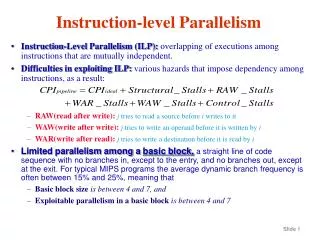
We now concentrate on promoting instruction level parallelism (ILP) in order to further improve pipeline performance ILP: amount of parallelism in a basic block of code code without branches, or code between branches given that branches make up about 15%-25% of all code in our MIPS examples

E N D
We now concentrate on promoting instruction level parallelism (ILP) in order to further improve pipeline performance ILP: amount of parallelism in a basic block of code code without branches, or code between branches given that branches make up about 15%-25% of all code in our MIPS examples a basic block may be between 4 and 6 instructions long question: of these 4-6 instructions, how many can be executed in parallel or overlapped fashion? if the number is low this argues for pipeline <= 4-6 stages otherwise, we will have to find ways to increase the available ILP in a basic block so we will also consider ways to extend ILP across blocks the more we can parallelize, the better our CPI performance will be, maybe even get CPI < 1 Instruction Level Parallelism
Consider the following loop This turns into the MIPS code on the right How much production can we get from this loop in a pipeline given that each iteration has a data hazard between the second L.S and the ADD.S a data hazard of 3 cycles between the ADD.S and S.S a data hazard between the DSUBI and the BNEZ a branch penalty The high-level language code is so concise that the machine code only has 8 instructions so there is not much ILP that can be exploited in the pipeline compiler scheduling can remove all of these hazards – can you figure out how? but this would not be true if we had a multiply instead of an add Example for(i = 1; i <= 1000; i++) x[i] = x[i] + y[i];
If 2 instructions are parallel, they can execute simultaneously in a pipeline without causing stalls But if 2 instructions are dependent then they are not parallel, and cannot be rearranged or executed in a pipeline at least, not without stalls or forwarding to safeguard the dependencies 3 forms of dependencies determine how code is parallelizable: data, name, control two instructions are data dependent if one instruction produces a result used by the other or one instruction is data dependent on an instruction which produces a result for the other these are RAW hazards data dependent instructions can only be executed in a pipeline if we can forward the results or insert stalls the likelihood of forwarding being successful depends on the pipeline depth and the distance between the instructions longer pipelines have a greater potential for stalls and for lengthier stalls name dependencies are WAW & WAR hazards these arise because of references to the same named location, not same datum name dependencies can be executed in parallel or overlap if we rename the locations Data vs. Name Dependencies
ADD.D is data dependent on L.D for F0, S.D is data dependent on ADD.D for F4 BNEZ is data dependent on DSUBI for R1 Both of these examples illustrate RAW hazards Name dependencies arise when 2 instructions refer to the same named item register, memory location But where there is no data dependency for instance, instruction i writes to name and instruction j reads from name but in between, the value of name is changed so these are not data dependences Instructions with name dependences may be executed simultaneously or reordered we can avoid name dependences through register renaming Data vs. Name Dependencies Register renaming can be done either statically or dynamically by a scoreboard-type mechanism
Antidependence instruction i writes to a name, instruction j reads from name, but j executes first (out of order) this can lead to a WAR hazard Output dependence instruction i and instruction j both write to the same name but j executes first (out of order) this can lead to a WAW hazard for output dependencies, ordering must be preserved There are data dependencies between L.D and ADD.D and between ADD.D and S.D, There are name dependencies between iterations of the loop that is, we use F0 in ADD.D and again in the next iteration but in the second iteration, F0 is referring to a different datum we can rename the register for the second iteration to remove name dependencies Forms of Name Dependence
Example Since there is a LC data dependence, the loop is not parallelizable although in the MIPS pipeline, the latency might be short enough to allow for unrolling and scheduling for(j=1;j<99;j++) { a[j] = b[j] * c[j+1]; // s1 c[j] = a[j+1] * s; // s2 a[j-1] = c[j] + b[j]; // s3 b[j+1] = a[j]; // s4 } • What are the dependencies in the following loop – for each, identify if the dependence is loop carried or not • is the loop parallelizable? Unrolling the loop would look like this: a[1] = b[1] * c[2]; c[1] = a[2] * s; a[0] = c[1] + b[1]; b[2] = a[1]; a[2] = b[2] * c[3]; c[2] = a[3] * s; a[1] = c[2] + b[2]; b[3] = a[2]; True (data) dependencies: b from s4 to s1 and s3 (LC) c from s2 to s3 (not LC) Output dependencies: a from s1 to s3 (LC) Anti dependencies: c from s2 to s1 (LC)
Control dependencies arise from instructions that depend on branches all instructions in a program have control dependencies except for the earliest instructions prior to any branch but here, we will refer to those instructions that are directly affected by a branch such as the then or else clause of an if-then-else statement or the body of a loop These dependencies must be preserved we preserve them by control hazard detections that cause stalls these stalls can be reduced through techniques such as filling the branch delay slots and loop unrolling instructions that are control dependent on a branch cannot be moved before the branch example: if(x!=0) x++; else y++; neither the if clause nor the else clause should precede the conditional branch of (x!=0)! an instruction not control dependent on a branch can not be moved after the branch Control Dependencies
Example • What are the control dependences from the code below? • Which statements can be scheduled before the if statement? • assume only b and c are used again after the code fragment d = d + 5 can be moved because d is only used again in a = b + d + e if the condition is true, and not used again if the condition is false a = b + d + e cannot be moved as it would affect a, thus impacting the outcome of the condition, and would affect the statement b = a + f if the condition were false e = e + 2 cannot be moved because it could alter a if the condition were false f = f + 2 cannot be moved because it could alter b and c incorrectly if the condition were true c = c + f cannot be moved because it will alter the condition and since c is used later, it may have the wrong value b = a + f cannot be moved since a or f might change if (a > c) { d =d + 5; a = b + d + e;} else { e = e + 2; f = f + 2; c = c + f; } b = a + f;
Consider the code to the right (equivalent to incrementing elements of an array) There is only so much scheduling that we can do to this code because it lacks ILP with forwarding, we need the following stalls 1 stall after L.D 2 stalls after ADD.D 1 stall after DSUBI 1 stall after BNEZ branch delay Pipeline Scheduling – Limitation to simplify problems in these notes, we will use new latencies which remove some of the stalls after FP *, /
Scheduling this Loop • We improve on the previous example by scheduling the instructions (moving them around) • move the DSUBI up to the first stall • this removes that stall • move the S.D after the BNEZ • this removes the last stall • this also reduces the stalls after the ADD.D to 1 since BNEZ does not need the result of the ADD.D • Only 1 stall now, after ADD.D! • Note: we can’t improve on this because of the limit of ILP in this loop Modify the displacement for the S.D since we have moved the DSUBI earlier
Loop Unrolling • Compiler technique to improve ILP by providing more instructions to schedule • As an advantage, loop unrolling consolidates loop mechanisms from several iterations into one iteration • we unroll the previous loop to contain 4 iterations so that it iterates only 250 times • we adjust the code appropriately: • new registers • alter memory reference displacements • change the decrement of R1 • the new loop is only slightly better because we have removed instructions, but once we schedule it, we will get a much better improvement Notice the change to the offsets Advantages: fewer branch penalties, provides more instructions for ILP Disadvantages: uses more registers, lengthens program, complicates compiler
Unrolled and Scheduled Version of the loop with no stalls • Now we use compiler scheduling to take advantage of extra ILP available: • with 4 L.Ds • we can remove all RAW hazards between a L.D and ADD.D by moving all L.Ds up earlier than the ADD.D • with 4 ADD.Ds • we can place them consecutively so we no longer have RAW hazards with the S.Ds • with 4 S.Ds • we move one between DSUBI and BNEZ and one after the BNEZ Notice the adjustment here
Original loop iterated 1000 times: each iteration takes 10 cycles* (5 instructions, 5 stalls) = 10,000 cycles Scheduled loop iterated 1000 times: each iteration takes 6 cycles* (5 instructions, 1 stall) = 6,000 cycles Unrolled and Scheduled loop iterates 250 times: each iteration takes 14 cycles after the first iteration (14 instructions, 0 stalls) = 3,500 cycles Speedup over original = 10,000 / 3,500 = 2.86 Speedup over scheduled but not unrolled = 6,000 / 3,500 = 1.71 all gains are from the compiler To perform unrolling and scheduling, the compiler must determine dependencies among instructions, how to move the loads and stores, adjust the offsets and the DSUBI determine that loop iterations are independent except for loop maintenance for instance, make sure that x[i] does not depend on x[i - 1] and compute a proper number of iterations that can be unrolled eliminate extra conditions, branches, decrements, and adjust loop maintenance code use different registers Results
Consider the code to the right assume 7 cycle multiply from appendix A Stalls: 1 after the second LD 7 after the MUL.D (or 6 if we can handle the structural hazard) 1 after the DSUBI 1 for the branch hazard We can schedule the code to remove just 3 stalls move the DSUBI after the second LD (removes 2 stalls) move the SD into the branch delay slot (removes 3 stalls) We will still have 5 stalls between the MUL.D and the SD we would place the stalls either after MUL.D or after DADDI but not after BNE – why? We can reduce the stalls by unrolling and scheduling the loop – how many times? how about 4 more times Another Example Loop: LD F0, 0(R1) LD F1, 0(R2) MUL.D F2, F1, F0 SD F2, 8(R2) DADDI R2, R2, #16 DSUBI R1, R1, #8 BNEZ R1, Loop
Loop: LD F0, 0(R1) LD F1, 0(R2) LD F3, 8(R1) LD F4, 16(R2) LD F6, 16(R1) LD F7, 32(R2) LD F9, 32(R1) LD F10, 48(R2) LD F12, 40(R1) LD F13, 64(R2) MUL.D F2, F1, F0 MUL.D F5, F3, F4 MUL.D F8, F6, F7 MUL.D F11, F9, F10 MUL.D F14, F12, F13 DADDI R2, R2, #80 DSUBI R1, R1, #40 SD F2, -72(R2) SD F5, -56(R2) SD F8, -40(R2) SD F11, -24(R2) BNEZ R1, Loop SD F14, -8(R2) Solution • Why unroll it 4 more times? • Consider • we will need 7 stalls or other instructions between the MUL.D and its SD • we have 3 operations that can go there (DADDI, DSUBI, BNEZ) but the branch cannot be followed by more than 1 instruction so we unroll the loop to create more instructions • so we need 4 more instructions to fill the remaining stalls • by unrolling the loop 4 times, we have 4 more MUL.Ds to fill those slots • we create more SDs, and only one (at most) can reside after the BNEZ • we move the DADDI and DSUBI to fill some of those slots and move them up early enough to remove the stall before the BNEZ • we arrange the code so that all LDs occur first, followed by all MUL.Ds, followed by our DADDI and DSUBI, followed by all of the SD with the BNE before the final SD • we also have to figure out the displacement offsets and how to adjust R1 and R2
Reducing Branch Penalties • We already considered static approaches to reduce the branch penalty of a pipeline • assume taken, assume not taken, branch delay slot • Now lets consider some dynamic (hardware) approaches • we introduce a buffer (a small cache) that stores prediction information for every branch instruction • if the branch was taken last time the instruction was executed (branch-prediction buffer) • if the branch was taken over the two times the instruction was executed (two-bit prediction scheme) • if the branch was taken and to where the last time the instruction was executed (branch-target buffer) • what the branch target location instruction was (branch folding) • if we can access this buffer to retrieve this information at the same time that we retrieve the instruction itself • we can then use the information to predict if and where to branch to while still in the IF stage, and thus remove any branch penalty!
Branch Prediction Buffer • The buffer is a small cache indexed by the low-order bits of the address of the instruction • the buffer stores 1 data bit pertaining to whether the branch was taken or not the last time it was executed (a 1 time history) • if the bit is set, we predict that the branch is taken • if the bit is not set, we predict that the branch is not taken • There is a draw-back to a 1-time history: • consider a for-loop which iterates 10 times with the branch prediction bit initially set to false (no branch) • first time through the loop, we retrieve the bit and predict that the branch will not be taken, but after the branch is taken, we set the bit • the next 8 iterations through the loop, we predict taken and so are correct • for the final iteration, the bit predicts taken, but it is not • even though the branch is taken 9 out of 10 times, our approach mispredicts twice, giving an accuracy of 80% • In general, loop branches are very predictable • they are either skipped or repeated many times • ideal accuracy of this approach = (# of iterations - 1) / # of iterations
We can enhance our buffer to store 2 bits to indicate for the last branch the combination of whether the branch was taken or not and whether we predicted taken or not (see the figure) if the 2-bit value >= 10 then predict taken after each branch, shift the value and tack on the new bit of whether the branch was taken or not We can generalize the 2-bit approach to an n-bit approach if the value >= 2^n / 2 then predict taken after each branch, shift to the left and add the new bit based on last branch It turns out that the n-bit approach is not that much better, so a 2-bit approach is good enough Using More Prediction Bits Here, we do not change the prediction after 1 wrong guess, we have to have 2 wrong guesses to change
The 1 or 2-bit approach only considers the current branch, but a compiler may detect correlation among branches consider the C code to the right the third branch will not be taken if the first two branches are both taken – if we can analyze such code, we can improve on branch prediction So we want to package together a branch prediction based not only on previous occurrences of this branch, but other branches’ behaviors this is known as a correlating predictor A (1, 2) correlating predictor uses the behavior of the last branch to select between 2 2-bit predictors a (m, n) correlating predictor uses the behavior of the last m branches to select between 2m n-bit predictors this is probably overkill, and in fact the (1, 2) predictor winds up offering a good prediction accuracy while only requiring twice the memory space of 2-bit predictors by themselves Correlating Predictors if(aa = = 2) aa = 0; if(bb = = 2) bb = 0; if(aa != bb) {…}
Tournament Predictors • The correlating predictor can be thought of as a global prediction whereas the earlier 1-bit or 2-bit predictors were local predictions • In some cases, local predictions are more accurate and in some cases global predictions are more accurate • A third approach, the tournament predictor, combines both of these by using yet another set of bits to determine which predictor should be used, the local or global • a 2-bit counter can be used to count the number of previous mispredictions • once we have two mispredictions, we switch from one predictor to the other • we might use static prediction information to determine which predictor we should start with • Figure 2.8 compares these various approaches and you can see that the tournament predictor is clearly the most accurate • prediction accuracy can be as low as about 2.8% on SPEC benchmarks • The Power5 and Pentium4 use 30K bits to store prediction information while the Alpha 21264 uses 4K 2-bit counters with 4K 2-bit global prediction entries and 1K 10-bit local prediction entries
Using Branch Prediction in MIPS • Notice that we are only predicting whether we are branching but not where we might branch to • we are fetching the branch prediction at the time we are fetching the instruction itself • in MIPS, the branch target address is computed in the ID stage, so we are predicting if we are branching before we know where to branch to (and we know for sure if we should branch in ID anyway) • therefore, there is no point in performing branch prediction (by itself) in MIPS, we also need to know where to branch too • the branch prediction technique is only useful in longer pipelines where branch locations are computed earlier than branch conditions Even with a good prediction, we don’t know where to branch too until here and we’ve already retrieved the next instruction
Branch-Target Buffers Send PC of current instruction to target buffer in IF stage If a hit (PC is in the table) then look up predicted PC and branch prediction If predict taken, update PC with the predicted PC otherwise increment PC as usual We predict branch location before we have even decoded the instruction to see that it is a branch! • In MIPS, we need to know both the branch condition outcome and the branch address by the end of the IF stage, so we enhance our buffer to include the prediction and if taken, the branch target location as well On a branch miss or misprediction, update the buffer by moving missing PC into buffer, or updating predicted PC/branch prediction bit
Consequence of this approach • If branch target buffer access yields a hit and the prediction is accurate, • then 0 clock cycle branch penalty! • what if miss or misprediction? • If hit and prediction is wrong, then 2 cycle penalty • one cycle to detect error, one cycle to update cache • If cache miss, use normal branch mechanism in MIPS, then 2 cycle penalty • one cycle penalty as normal in MIPS plus one cycle penalty to update the cache
Branch Folding • Notice that by using the branch target buffer • we are fetching the new PC value (or the offset for the PC) from the buffer • and then updating the PC • and then fetching the branch target location instruction • Instead, why not just fetch the next instruction? • In Branch folding, the buffer stores the instruction at the predicted location • If we use this scheme for unconditional branches, we wind up with a penalty of –1 (we are in essence removing the unconditional branch) • Note: for this to work, we must also update the PC, so we must store both the target instruction and the target location • this approach won’t work well for conditional branches
For branch target buffer: prediction accuracy is 90% branch target buffer hit rate is 90% branch penalty = hit rate * percent incorrect predictions * 2 cycles + (1 - hit rate) * 2 cycles = (90% * 10% * 2) + (1 - 90%) * 60% * 2 = .38 cycles Using delayed branches (as seen in the appendix notes), we had an average branch penalty of .3 cycles so this is not an improvement, however for longer pipelines with greater branch penalties, this will be an improvement, and so could be applied very efficiently For branch folding: Assume a benchmark has 5% unconditional branches A branch target buffer for branch folding has a 90% hit rate How much improvement is gained by this enhancement over a pipelined processor whose CPI averages to 1.1? This processor has CPI = 1 + .05 * .9 * (-1) + .05 * .1 * 1 = 0.96 (a CPI < 1!) This processor is then 1.1 / 0.96 = 1.15 or 15% faster Examples
Return Address Predictors • We have a prediction/target buffer for conditional branches, what about unconditional branches? • GO TO type statements can be replaced by branch folding, but return statements are another matter • several functions could call the same function, so return statements are unconditional branches that could take the program to one of several locations • one solution is to include a stack of return addresses • if the stack size <= depth of function calls, this works well, but if not, we begin to lose addresses and so the “prediction” of the return value decreases from an idea of 100% accurate • NOTE: the return values are already stored in the run-time stack in memory, we are talking about adding a return stack in cache • figure 2.25 demonstrates the usefulness of different sized caches where an 8-element cache yields 95% accuracy in prediction
Integrated Fetch Units • With the scoreboard, we separated the instruction fetch from the instruction execution • We will continue to do this as we explore other dynamic scheduling approaches • In order to perform the instruction fetches, coupled with branch prediction, we add an integrated fetch unit • a single unit that can fetch instructions at a fast rate and operates independently of the execution units • An integrated fetch unit should accomplish 3 functions: • branch prediction (possibly using a branch target buffer) constantly predicting whether to branch for the next instruction fetch • instruction prefetch to fetch more than 1 instruction at a time (we will need this later when we explore multiple issue processors) • memory access and buffering to buffer multiple instructions fetched by more than one cache access
Sample Problem #1 • Using the new latencies from chapter 2 and assuming a 5-stage pipeline with fowarding available and branches completed in the ID stage • determine the stalls that will arise from the code as is • unroll and schedule the code to remove all stalls • note: assume that no structural hazard will arise when an FP ALU operation reaches the MEM stage at the same time as a LD or SD • if the original loop were to iterate 1000 times, how much faster is your unrolled and scheduled version of the code? • From the code below Loop: LD R2, 0(R1) LD F0, 0(R2) ADD.D F2, F0, F1 LD F3, 8(R2) MUL.D F4, F3, F2 SD F4, 16(R2) DSUBI R1, R1, #4 BNEZ R1, Loop
Solution Loop: LD R2, 0(R1) LD F0, 0(R2) LD R3, 4(R1) LD F5, 4(R3) ADD.D F2, F0, F1 ADD.D F6, F5, F1 LD F3, 8(R2) LD F7, 8(R3) MUL.D F4, F3, F2 MUL.D F8, F7, F6 DSUBI R1, R1, #8 SD F4, 16(R2) BNE R1, Loop SD F8, 16(R2) • Stalls: • 1 after each LD (3 total) • 1 after ADD.D • 2 after MUL.D • 1 after DSUBI • 1 after the branch • Unroll: • the greatest source of stalls will be after the MUL.D, however we can insert the DSUBI to take up one spot, so we need 1 additional instruction there • we will unroll the loop 1 additional time • Speedup: • original loop takes 14 cycles (excluding the first iteration) • new loop takes 14 cycles for 2 iterations • therefore, there is a 2 times speedup
Sample Problem #2 • MIPS R4000 pipe has 8 stages, branches determined in stage 4 • make the following assumptions: • the only source of stalls is from branches • we modify the MIPS R4000 to compute the branch target location in stage 3 but conditions are still computed in stage 4 • the compiler schedules 1 neutral instruction the branch delay slot 80% of the time and that aside from the branch delay slot, we implement assume not taken • if a benchmark consists of 5% jumps/calls/returns and 12% conditional branches, and assuming that 67% of all conditional branches are taken, what is the CPI of this machine?
Solution • CPI = 1 + branch penalty / instruction • unconditional branches will have a penalty of 1 if branch delay slot is filled or 2 if branch delay slot is not filled since we know where to branch to at the end of stage 3 • conditional branches will have a penalty of 0 if we do not take the branch, 2 if we take the branch and the branch delay slot is filled, or 3 if we take the branch and the branch delay slot is not filled • branch penalty / instruction = 5% * (80% * 1 + 20% * 2) + 12% * 67% * (80% * 2 + 20% * 3) = .237 • CPI = 1.237
Assume in our 5-stage MIPS pipeline that we have more complex conditions so that we can determine where to branch in stage 2 but we don’t know if we are branching until the 3rd stage We want to enhance our architecture with a prediction buffer with a hit rate of 92% and accuracy of 89% or a target buffer with a hit rate of 80% (the target buffer has to store more, so it will store less entries) and accuracy of 82% We retrieve the prediction/target info in the IF stage if we guess right, we have a 0 cycle penalty but on a miss or miss-prediction, we will have a 1 cycle penalty to update the buffer on top of any branch penalty Which buffer should we use assuming that our benchmark we are testing has 5% jump/call/return and 12% conditional branch? Sample Problem #3
Solution • Miss or miss-prediction on unconditional branch has 1 cycle penalty + 1 cycle buffer update • Miss or miss-prediction on conditional branch has 2 cycle penalty + 1 cycle buffer update • prediction Buffer: • CPI = 1 + .08 * .05 * 2 + .08 * .12 * 3 + .92 * .11 * .05 * 2 + .92 * .11 * .12 * 3 = 1.083 • target Buffer: • CPI = 1 + .20 * .05 * 2 + .20 * .12 * 3 + .20 * .18 * .05 * 2 + .20 * .18 * .12 * 3 = 1.109 • so the prediction buffer, in this case, gives us a better performance