Download
1 / 43
460 likes | 893 Vues
Image Classification. Convolutional networks - Why. Convolutions Reduce parameters Capture shift-invariance: location of patch in image should not matter Subsampling Allows greater invariance to deformations Allows the capture of large patterns with small filters.

E N D
Convolutional networks - Why • Convolutions • Reduce parameters • Capture shift-invariance: location of patch in image should not matter • Subsampling • Allows greater invariance to deformations • Allows the capture of large patterns with small filters
How to do machine learning • Create training / validation sets • Identify loss functions • Choose hypothesis class • Find best hypothesis by minimizing training loss
How to do machine learning Multiclass classification!! • Create training / validation sets • Identify loss functions • Choose hypothesis class • Find best hypothesis by minimizing training loss Negative log likelihood for multiclass classification
Negative log likelihood for multiclass classification • Often represent label as a ``one-hot’’ vector y • y = [0, 0, …, 1,… 0] • yk = 1 if label is k, 0 otherwise
Building a convolutional network conv + relu + subsample conv + relu + subsample linear 10 classes average pool conv + relu + subsample
Building a convolutional network 5x5 conv, no subsample 5x5 conv, subsample by 2 Linear 6 6 10 84 120 16 Linear(classifier) Flatten+ Linear 5x5 conv, subsample by 2
Training the network Overfitting
Controlling overfitting in convolutional networks • Reduce parameters? • Increase dataset size? • Automatically by jittering examples - “Data augmentation”
Controlling overfitting in convolutional networks • Dropout: Internally create data augmentations • Randomly zero out some fraction of values before a layer • Can be thought of as per-layer data augmentation • Typically applied on inputs to linear layers (since linear layers have tons of parameters)
Dropout Without dropout Train error: 0% Test error: 1% With dropout Train error: 0.7% Test error: 0.85%
ImageNet • 1000 categories • ~1000 instances per category Olga Russakovsky*, Jia Deng*, Hao Su, Jonathan Krause, Sanjeev Satheesh, Sean Ma, Zhiheng Huang, Andrej Karpathy, Aditya Khosla, Michael Bernstein, Alexander C. Berg and Li Fei-Fei. (* = equal contribution) ImageNet Large Scale Visual Recognition Challenge. International Journal of Computer Vision, 2015.
ImageNet • Top-5 error: algorithm makes 5 predictions, true label must be in top 5 • Useful for incomplete labelings
7-layer Convolutional Networks 19 layers 152 layers
Deeper is better 7 layers 16 layers
Deeper is better Alexnet VGG16
The VGG pattern • Every convolution is 3x3, padded by 1 • Every convolution followed by ReLU • ConvNet is divided into “stages” • Layers within a stage: no subsampling • Subsampling by 2 at the end of each stage • Layers within stage have same number of channels • Every subsampling double the number of channels
Example network 5 5 10 10 20 20
Challenges in training: exploding / vanishing gradients • Vanishing / exploding gradients • If each term is (much) greater than 1 explosion of gradients • If each term is (much) less than 1 vanishing gradients
Residual connections • In general, gradients tend to vanish • Key idea: allow gradients to flow unimpeded
Residual connections • In general, gradients tend to vanish • Key idea: allow gradients to flow unimpeded
Residual block Conv + ReLU Conv+ReLU
Residual connections • Assumes all zi have the same size • True within a stage • Across stages? • Doubling of feature channels • Subsampling • Increase channels by 1x1 convolution • Decrease spatial resolution by subsampling
The ResNet pattern • Decrease resolution substantially in first layer • Reduces memory consumption due to intermediate outputs • Divide into stages • maintain resolution, channels in each stage • halve resolution, double channels between stages • Divide each stage into residual blocks • At the end, compute average value of each channel to feed linear classifier
Transfer learning with convolutional networks Linear classifier Horse Trained feature extractor
Transfer learning with convolutional networks • What do we do for a new image classification problem? • Key idea: • Freeze parameters in feature extractor • Retrain classifier Linear classifier Trained feature extractor
Why transfer learning? • Availability of training data • Computational cost • Ability to pre-compute feature vectors and use for multiple tasks • Con: NO end-to-end learning
Finetuning Horse
Finetuning Bakery Initialize with pre-trained, then train with low learning rate
Receptive field • Which input pixels does a particular unit in a feature map depends on convolve with 3 x 3 filter
Receptive field convolve with 3 x 3 filter convolve with 3 x 3 filter 3x3 receptive field 5x5 receptive field
Receptive field convolve with 3 x 3 filter, subsample
Receptive field convolve with 3 x 3 filter, subsample by factor 2 convolve with 3 x 3 filter 3x3 receptive field 7x7 receptive field: union of 9 3x3 fields with stride of 2
Visualizing convolutional networks • Take images for which a given unit in a feature map scores high • Identify the receptive field for each. Rich feature hierarchies for accurate object detection and semantic segmentation. R. Girshick, J. Donahue, T. Darrell, J. Malik. In CVPR, 2014.
Visualizing convolutional networks II • Block regions of the image and classify Visualizing and Understanding Convolutional Networks. M. Zeiler and R. Fergus. In ECCV 2014.
Visualizing convolutional networks II • Image pixels important for classification = pixels when blocked cause misclassification Visualizing and Understanding Convolutional Networks. M. Zeiler and R. Fergus. In ECCV 2014.