Download
1 / 31
340 likes | 510 Vues
Pre-Processing of CCD Data. ASTR 3010 Lecture 9 Textbook Chap 9. Raw CCD images. Nearly all astronomy data are distributed as FITS (Flexible Image Transport System) files. Each FITS file consists of header + data (Header Data Units, HDUs )

E N D
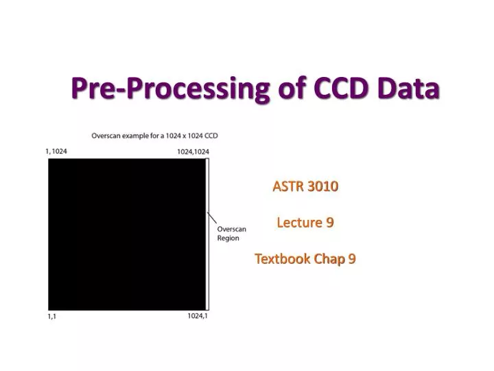
Pre-Processing of CCD Data ASTR 3010 Lecture 9 Textbook Chap 9
Raw CCD images • Nearly all astronomy data are distributed as FITS (Flexible Image Transport System) files. • Each FITS file consists of header + data (Header Data Units, HDUs) • header: 80 characters long fixed width info. No limit on the number of headers. Each header line has a keyword and value (and optionally a comment) IMAGETYP= 'OBJECT ' / Type of Object • Data: binary format of actual data • There can be multiple extension several HDUs multi-extension FITS (MEF)
Sample FITS Header Header listing for HDU #1: SIMPLE = T / Fits standard BITPIX = 16 / Bits per pixel NAXIS = 2 / Number of axes NAXIS1 = 1172 / Axis length NAXIS2 = 1026 / Axis length EXTEND = F / File may contain extensions BSCALE = 1.000000E0 / REAL = TAPE*BSCALE + BZERO BZERO = 3.276800E4 / DATAMIN = 5.370000E2 / Minimum data value DATAMAX = 1.255900E4 / Maximum data value OBJECT = 'HD 189933' / Name of the object observed IMAGETYP= 'OBJECT ' / Type of picture (object, dark, etc.) DETECTOR= 'Tek2K_3 ' / Detector (CCD type, photon counter, etc.) PREFLASH= 0.000000 / Preflash time in secs CCDSUM = '1 1 ' / On chip summation (X,Y) DATE-OBS= '19/08/99' / Date (dd/mm/yy) of observation UT = ' 3:24:48.00' / UT of TCS coords OBSERVAT= 'CTIO ' / Origin of data TELESCOP= 'CTIO 0.9 meter telescope' / Specific system . . . RA = '20:04:25.40' / right ascension (telescope) DEC = '-45:02:14.30' / declination (telescope) EPOCH = 2000.0 / epoch of RA & DEC ZD = 15.7 / zenith distance (degrees) HA = '00:25:21.1' / hour angle (H:M:S) ST = '20:29:47.60' / sidereal time AIRMASS = 1.039 / airmass EXPTIME = 20.000 / Exposure time in secs INSTRUME= 'cfccd' / cassegrain direct imager FILTER2 = 'b' / Filter in wheel two . . . END
Handling FITS file • FITS file I/O • IRAF : dataio • IDL : readfits/writefits etc. • Python: pyfits import pyfits data = pyfits.getdata(‘file1.fits’) primary HDU data2 = pyfits.getdata(‘file1.fits’,2) 2nd extension data2 = pyfits.getdata(‘file1.fits,ext=2) header = pyfits.getdata(‘file1.fits’) # get both data and header from a single command data, hdr = pyfits.getdata(‘file1.fits’, header=True) # access a specific keyword print hdr[‘ra’] # add your own keyword hdr.update(‘TESTKEY’, ‘my first keyword’) ..
Displaying FITS images • Iraf: ximtool • IDL: atv … • We will use DS9 http://hea-www.harvard.edu/RD/ds9/
Accessing DS9 from Python import pyfits from ds9 import * data=pyfits.getdata(‘file1.fits’) d=ds9() d.set_np2arr(data) will not work, why? d.set_np2arr( transpose(data) ) numpy addresses [y,x] instead of [x,y] # Better way to do is … hdus = pyfits.open(‘file1.fits’) d.set_pyfits(hdus) even accessing to the WCS (world coordinate system).
A Handful of Important CCD frames • Bias : zero second exposure showing detector electronic noise pattern etc. • Dark : data taken with shutter closed to eliminate dark current. • Flat : uniformly illuminated data to eliminate pixel-to-pixel sensitivity variation (QE variation) dome flats + sky flats • Badpixel masks : To interpolate over badpixels
Typical Steps of CCD pre-processing Insufficient calibration files (bias, darks, flats) can lead into noisier data!! Check the noise statistics before and after to decide if you want to apply the above steps!!
Bias frames • The bias frame is a CCD image with an exposure time of zero seconds and shutter closed (i.e. a dark frame with no exposure time). In this way the CCD is simply readout. The interest about the bias frame resides in the determination of the underlying fixed noise pattern (called "bias level") and the readout noise within each data frame. • Why bias? fat zero for ADC operation (Ex.) for a 16bit ADC, if a count is -5 due to a noise recorded as 65530
Bias image • Example
Overscan Correction and CCD frame trimming • Overscan region: electric voltage of the CCD can fluctuate over time • Cut off the overscan region Show: Actual example of the overscan region in Python
Readout noise • Can be best estimated from two bias frames • Make a plot of bias1 – bias2 √2 times the readout noise • Readout noise = FWHM=2.354σ
Dark Frames • The dark frame is taken with the same exposure time, at the same operational temperature, as the raw image, but with the shutter closed. It records the dark current in the CCD chip. • Dark correction = dark subtraction science target image – combined dark frames
Flat Frames • The flat field image is recorded by pointing the instrument towards a uniformly illuminated surface. It records differences in the sensitivity of pixels, and vignetting in the optical path. A typical flat frame
CCD and Infrared Array Data pre-processing • Both detectors show “additive” and “multiplicative” effects • Additive class • electronics pattern noise (“bias effects”) • charge trapping • interference fringes • Multiplicative class • quantum efficiency variation across the array • transmission of optics and coatings • thickness variations of photoelectron generating layer
Recipe for reduction and calibration of astronomical data • subtract bias • subtract dark: most CCDs exhibit some dark current leading to “electronic” pollution during long exposures. To correct this, the “median image” of many long (bias-subtracted) dark exposures must be subtracted from object frames. • Divide by flat-field: bias-corrected, dark-subtracted, normalized flat-fields are median combined to form a master flat. Then this master flat is divided into the dark-corrected object frames to calibrate for QE variation from pixel to pixel. • Subtracting fringe frame; sky subtraction • Interpolate over bad pixels: using bad pixel map or dithering on the sky. • Remove cosmic ray events • Registration of frames and median filtering
Fringes • in far-red, or near-infrared images, variable sky mission lines are causing an interference pattern due to multiple reflection within the detector silicon layer. Can be removed by adaptive modal filtering for a set of images. • Single image with a fringe Fourier Transform technique
Cosmic Ray hits removal • Two ways: using multiple frames versus single frame based. • Left: No Treatment • Right: CR removal by xzap method
Caveats with Flat fields… • Dome flats : illumination (pattern and color) of the dome light can be quite different from the night sky. • Twilight flats: flats taken during twilights color of twilight sky can be quite different from the color of science targets. Gradient in twilight (horizon is brighter!) • Flats are color dependent!! i-band green red
To remove a slow variation across the detector • U-band twilight flat (2.0sec) taken with the UGA Physics telescope unfocused dust ring
To remove a slow variation across the detector • U-band twilight flat (0.5sec) taken with the UGA Physics telescope box=ones( (101,101) ) sm=convolve2d(flat, box)
To remove a slow variation across the detector • U-band twilight flat (0.5sec) taken with the UGA Physics telescope ÷ box=ones( (101,101) ) sm=convolve2d(flat, box) new_flat = flat/sm
UGA Physics telescope flats U B V R I
Creating a bad pixel map • Manually? possible, and some meticulous peoples are doing it • Using two different flats with different illumination levels. average count=200,000 average count=300,000 Keck NIRC camera flats (taken in 2006)
Creating a bad pixel map ÷ set pixels that are deviant from the mean as “bad”
Bad pixel map ratio = flat1 / flat2 bads = where (ratio > 1.65 || ratio < 1.35) badpixel_map = zeros( (256,256) ) badpixel_map[bads] = 1
Using UGA Physics flats… • ratioed image (e.g., 11 median combined U-flats of high illumination – 11 median combined U-flats of low illumination) So, bad pixels are with ratio > 5.7 or ratio < 5.4
UGA Physics Telescope CCD bad pixel map bpm=zeros( ratio.shape ) bads=where( (ratio>5.7) | (ratio<5.4)) bpm[bads] = 1 Nbad = 404 pixels
Example of bad pixel correction • Bad pixel interpolation with a Gaussian kernel after before
Automatic bias, dark, CR, sky subtraction!! • observation with random offsets Next Lecture!!
In summary… Important Concepts Important Terms Overscan FITS, header, HDU Bias, dark, flat dome flat twilight flat sky flat • Need for bias & overscan region • Pre-processing of CCD data • Combine multiple frames of the same kind (why?) • Bad pixel correction • Pros and cons of different flats • Fringe • Chapter/sections covered in this lecture : 9