Download
1 / 31
390 likes | 868 Vues
The Endowment Effect. The Key Papers. Kahneman and Tversky , Econometrica , 1979. Kahneman , Knetsch and Thaler , Journal of Political Economy , 1990. Kahneman , Knetsch and Thaler , Journal of Economic Perspectives , 1991.

E N D
The Key Papers Kahneman and Tversky, Econometrica, 1979. Kahneman, Knetsch and Thaler, Journal of Political Economy, 1990. Kahneman, Knetsch and Thaler, Journal of Economic Perspectives, 1991. List, “Does Market Experience Eliminate Market Anomalies” Quarterly Journal of Economics, 2003.
A good review of WTA/WTP Studies By John K. Horowitz and Kenneth E. McConnell from the Journal of Environmental Economics and Management Vol. 44: 426-447.
The Mug (Bottle of Pop) Experiment Half the class randomly endowed with a good. Students endowed with the good were asked to express their willingness to accept (WTA) – the minimum price at which they would be willing to sell. Students without good were asked to express their willingness to pay (WTP) – the maximum price at which they would be willing to buy.
The Mug (Bottle of Izze) Experiment Past Results: Average WTA = $23.25/15 = $1.55 Average WTP = $12.00/13 = $0.92 Other Examples: Egg McMuffin Average WTA = $1.97 Average WTP = $0.89 T-shirts Average WTA = $6.5Average WTP = $2.2
What IS the Endowment Effect? The observation that people often demand much more to give up an object than they would be willing to pay to acquire it (Thaler, JEBO 1980).
Anomaly? Why is this “endowment effect” a puzzle from the perspective of neoclassical economics? What SHOULD we expect?
The Market Price $2.5 $2.0 $1.5 $1.0 $0.5 Demand $0 2 4 6 8 10 12 14 Quantity
The Market Price $2.5 Supply $2.0 $1.5 Price D S$1.25 5 6$1.00 8 5 $1.0 $0.5 Demand $0 2 4 6 8 10 12 14 Quantity Q*
We expect that… When a market clears, the objects will be owned by those subjects who value them most. Imagine you have two groups of people – those who love the object and those who hate it. If the good is distributed randomly, on average, half of those who love it will get it and half that don’t will also get it. Those who don’t love it should trade with those who love it and both will be made better off…. 50% of the object should be traded The willingness to pay for a good and minimum compensation demanded for the same entitlement (willingness to accept) should be negligible.
However The anomaly is a manifestation of the assymetry of value that Kahneman and Tversky (1984) call “loss aversion” Or, the disutility of giving up an object is greater than the utility associates with acquiring it.
Implications of the Endowment Effect on Markets Q*with EE < Q* without EE An implication of this asymmetry is that if a good is evaluated as a loss when it is given up and as a gain when it is acquired, loss aversion will, on average induce higher dollar value for owners than for potential buyers… This will reduce the set of mutually acceptable trades (Kahneman, Knetsch and Thaler, JPE 1990).
Implications Price $2.5 $2.0 Supply (Endowment Effect) $1.5 Supply (No Endowment Effect) $1.0 $0.5 Demand $0 2 4 6 8 10 12 Quantity
Now let’s explore the EE on Indifference Curves What does prospect theory imply for individual indifference curves?
Value Losses Gains
Review: Three Features of the Value Function It is defined on deviations from a reference point (gains and losses, not wealth) It is concave for gains (implying risk aversion) and convex for losses (implying risk seeking) It is steeper for gains than losses (loss aversion)
Conventional Preferences • People can judge which of two options is preferable (or equally preferred). • Preference ordering must be transitive (not true of love) • People must be able to trade off values against each other. • “Maintained States” are carriers of utility (Tversky and Kahneman).
Conventional Preferences Marginal Rate of Substitution (MRS) MUX = - MUY Example: U(X) = log(X) & U(Y) = log(Y) MRS = - Y/X
Violation of Assumption 1: Indifference Curves cannot cross If an individual owns x and is indifferent between keeping it and trading for y, then when owning y, the individual should be indifferent about trading it for x. If loss aversion is present, this assumption will not hold.
Knetsch (1990) Tested this Assumption One group of subjects received 5 medium priced ball point pens Another group of subjects received $4.50 Each group was made a series of offers which they could accept or reject. The offers were designed to identify the subject’s indifference curves showing willingness to trade between pens and dollars. Subjects were notified that one of the accepted offers would be selected at random to determine the subject’s payment.
Knetch’s Indifference Curves There was a pronounced endowment effect The pen was preferred by 56 percent of those endowed with it, but only 24 percent of the other subjects chose a pen
More Implications Indifference curves are drawn without reference to current endowments. One explanation for the EE is that people have reference-dependent preferences, defined over changes in the consumption of goods rather than over levels.
Implications:Reference-Dependent Preferences Y Endowment Point Normal Indifference Curve X
More Implications Any difference between equivalent and compensating variation assessments of welfare changes is in practice ignored
“Kinky” Preferences: Insensitivity to price changes Y (PX/PY) Endowment Point Inertia X Endowment Point
Implications: Price StickinessSlow Adjustment to Equilibrium P S Genegove and Mayer (2001) – List prices of Boston condos are highly correlated with the original purchase price. People should regard the original purchase price as a sunk cost and ignore it. Original purchase price = $300,000 Current Market Price = $275,000 Listing Price = $295,000 P*1 P*2 D D’ Q
Implications: The Coase Theorem Coase Theorem: the allocation of resources will be independent of the assignment of property rights when costless trades are possible. Kahneman, Knetsch and Thaler (1990): if the MRS between two goods is affected by endowment, the individual who is assigned the property right to a good will be more likely to retain it.