Download
1 / 44
480 likes | 727 Vues
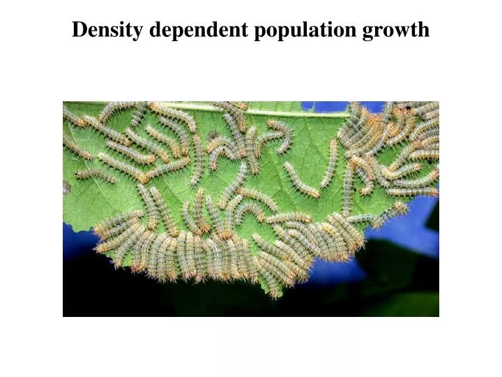
Density dependent population growth. Assumptions of exponential growth. Assumptions of our simple model: No immigration or emigration Constant b and d No random variation Constant supply of resources No genetic structure (all individuals have the same birth and death rates)

E N D
Assumptions of exponential growth • Assumptions of our simple model: • No immigration or emigration • Constant b and d • No random variation • Constant supply of resources • No genetic structure (all individuals have the same birth and death rates) • No age or size structure (all individuals have identical b and d ) N t
Are b and d really constant? The exponential model assumes this But for many organisms b and d are DENSITY DEPENDENT b b r d Rate Rate d r Population size, N Population size, N
Example 1: Northern Gannet Northern Gannet Morus bassunus Northern Gannet colony • Pelagic, fish eating seabird • Live in colonies ranging in size from 100 to 10,000 birds • Data on historical population sizes is available for nine colonies/populations
Example 1: Northern Gannet (Lewis et al 2001; Nature) • Studied 17 colonies • Collected data on current colony size • Collected data on historical colony size
Example 1: Northern Gannet (Lewis et al 2001; Nature) • Plotted Log[(1994 colony size)/ (1984 colony • size)] against Log[1984] colony size • Linear regression showed that small colonies • grew more rapidly (per capita) than did large • colonies Populations which grew Populations which shrank What caused this reduction in growth rate for large colonies?
Example 1: Northern Gannet (Lewis et al 2001; Nature) • Measured the duration of feeding flights • Plotted duration of feeding flights against • colony size • Linear regression revealed that the • duration of feeding flights increases with • colony size • Suggests that the reduction in growth • rates observed in large colonies results • from food scarcity
Example 2: Light Red Meranti • Dominant canopy tree • Found in the rain forests of Malaysia • Threatened by deforestation Light Red Meranti (Shorea quadrinervis)
Example 2: Light Red Meranti (Blundell and Peart, 2004. Ecology) • Studied 16 80m diameter plots in Gunung Palung National Park • 8 plots had a low density of the focal species • 8 plots had a high density of the focal species Gunung Palung National Park
Example 2: Light Red Meranti (Blundell and Peart, 2004. Ecology) • Measured the survival of juvenile trees in low and high density populations • Juvenile trees survived better in populations with low adult density
Example 2: Light Red Meranti (Blundell and Peart, 2004. Ecology) • Estimated the growth rate of the • populations based on data collected • from juvenile trees • Plotted estimated population growth • rate against the number of adults in each • population • Linear regression showed that growth • rate decreases as the number of adults • increases
These examples show that b and d depend on N Death rate, d Birth rate, b Death rate Birth rate Population density, N Population density, N a measures how rapidly the birth rate decreases with increasing density c measures how rapidly the death rate increases with increasing density
This leads to the logistic model We can start from the same basic framework as the exponential model: In 1838, Verhulst realized that density dependence can be incorporatedsimply by replacing b and d with functions that depend on N:
The logistic model Rearranging this equation a bit, gives the following: Several of the terms in this equation have a ready biological interpretation: This r is the maximum intrinsic rate of increase for a population. This maximum occurs only when the population is very small. At this point, the population experiences approximately exponential growth. This K is the carrying capacity of the environment, it tells us the maximum number of individuals that the environment can support.
Where is the K of a population? b d Rate dN/dt Population size, N This point, where the birth and death rates become equal (b=d), is the carrying capacity, K, of the population.
The logistic model Ultimately, the logistic model is written in this way: We can easily find the equilibria of the logistic by setting the rate of change in population size equal to zero: What are the equilibria?
The logistic model Equilibrium 1: N = 0 dN/dt Population size decreases Population size, N Equilibrium 2: N = K
Comparing the logistic and exponential models Exponential dN/dt Logistic Population size, N The exponential model has only a single equilibrium, N = 0 The logistic model has the additional equilibrium, N = K
Behavior of the logistic model K = 100 Population size, N Time, t With the logistic model, all initial population sizes end up converging on the carrying capacity, K.
Practice Problem Wolverine (Gulo gulo) • The question: How likely it is that a small (N0 = 36) population of wolverines will persist for 80 years without intervention? • The data: r values across ten replicate studies
How could we use the logistic model? • Predicting “maximum sustainable yield” • Understanding how harvested populations can suddenly collapse
Estimating maximum sustainable yield The question: at what density should the fish population be maintained in order to maximize the long term yield? ? ? ? K 0 Population size after harvesting
Why is this the ‘correct’ solution? K = 500 dN/dt N
Understanding the collapse of harvested populations Peruvian anchovy In 1970, a group of scientists estimated that the sustainable yield was around 9.5 million tons, a number that was currently being surpassed (see Figure 4). Shortly thereafter the fishery collapsed and did not recover. WHY?
Understanding the collapse of harvested populations • How could you modify the logistic model to account for the constant removal of some number of individuals? ?
Understanding the collapse of harvested populations • What does this new model tell us? h = 1 K K What happens below this density? What happens below this density? Does this population reach K? Does this population reach K?
Understanding the collapse of harvested populations • Now, add in a disturbance (e.g., El Nino), as happened with the Peruvian Anchovy h = 1 Disturbance If a disturbance reduces the number of individuals below this point, what happens?
Summarizing dynamics of harvested populations Fishing No disturbance No fishing No disturbance Population size Fishing & Disturbance No fishing Disturbance Time Time
Summarizing dynamics of harvested populations Fishing & Disturbance Population size Time If fishing pressure is removed, would these populations recover?
Maybe so… Maybe not • Demographic stochasticity • Genetic drift and inbreeding • Allee effects
Allee effects • Positive density dependence at low densities • First described by W. C. AlleeandEdith S. Bowen in 1932 • Caused by social processes which operate more efficiently with more individuals • e.g., Finding mates, group defense against predators, group pursuit of prey
Predator induced Allee effects Bourbeau-Lemieux et al. (2011) • Studied a population of bighorn sheep in Sheep River Provincial Park (Alberta) • Explored how cougar predation influenced offspring recruitment Cougar (Puma concolor) Bighorn sheep (Oviscanadensis) In Sheep River Provinical Park
Impact of predation greater in small populations • During periods of intense cougar predation: • Fewer lambs survived to weaning in small populations • Fewer lambs survived the winter in small populations • Suggests Allee effects caused by cougar predation • May be because individual predation risk increases as sheep population size falls making the sheep nervous which causes them to feed less, use poor quality habitat, and nurse less Survival to weaning Overwinter survival
Do real populations grow logistically? Connochaetes taurinas Salix cinerea Some appear to… Rhizoperthadominica From Begon et. al. 1996
But others do not: a classic experiment with blowflies Nicholson (1957)
A classic experiment with blowflies Nicholson (1957) • Fed cultures of blowflies a fixed amount of beef liver for the larvae daily • Fed cultures an ample supply of sugar and water for the adults • Followed the number of flies in the various experimental cages
50g 25g The result was clearly not logistic growth!
What happened? Imagine that the liver can support 6 larvae, and that each adult produces two eggs N = 2 N = 4 2 adults die This population is below carrying capacity This population is above carrying capacity all larvae live 2 eggs 2 adults die all larvae die N = 4 N = 2 2 adults die all larvae live This population is above its carrying capacity This population is below carrying capacity
What happened? • One of the assumptions of the logistic model was violated • Linear density dependence • No genetic structure • No age structure • No immigration or emigration • No time lags
50g 25g Could time lags have caused the cycles?
The discrete logistic equation One common way to generate time lags is to have discrete generations (e.g., annual plants, many insects, etc…) In these situations population growth is described by a discrete version of the logistic model:
The discrete logistic equation The carrying capacity, K, is set to 1000 in each of these cases r = .5 r = 2.4 Population size, N r = 2.7 r = 1.9 Generation # Time lags produced by discrete generations can generate cycles and even chaos
Practice question In order to identify the importance of density regulation in a population of wild tigers, you assembled a data set drawn from a single population for which the population size and growth rate of are known over a ten year period. This data is shown below. Does this data suggest population growth in this tiger population is density dependent? Why or why not? What problems do you see with using this data to draw conclusions about density dependence?