Download
1 / 32
320 likes | 471 Vues
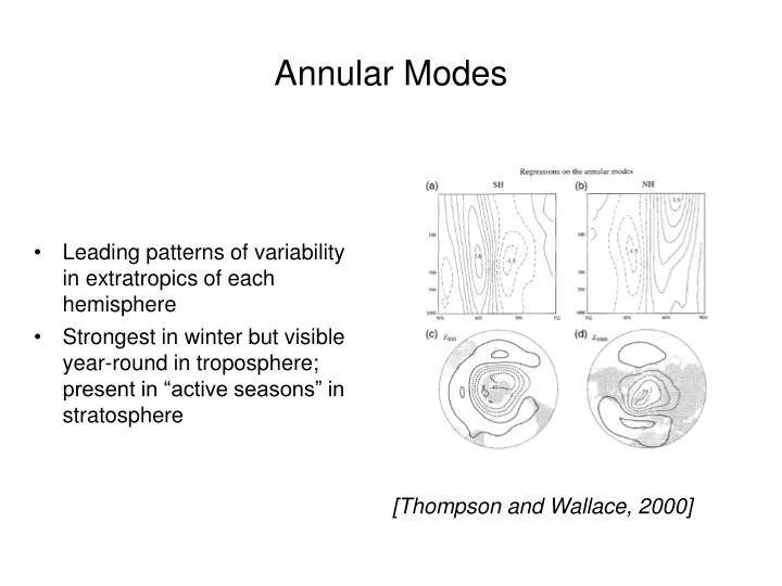
Annular Modes. Leading patterns of variability in extratropics of each hemisphere Strongest in winter but visible year-round in troposphere; present in “active seasons” in stratosphere. [Thompson and Wallace, 2000]. Climate forcings and annular modes.

E N D
Annular Modes • Leading patterns of variability in extratropics of each hemisphere • Strongest in winter but visible year-round in troposphere; present in “active seasons” in stratosphere [Thompson and Wallace, 2000]
Climate forcings and annular modes Tropospheric response to ozone depletion [Thompson & Solomon, 2002] GCM response to global warming [Kushner et al., 2001]
Response to altered stratospheric radaiative state[Kushner & Polvani 2004]
The fluctuation – dissipation theorem[Leith and others] response projection of variance of autocorrelation time forcing unforced mode of unforced mode
Response to altered stratospheric radaiative state[Kushner & Polvani 2004]
Haynes et al (1991) Instantaneous (Eliassen) response Long-time (steady, “downward control”) response ut χ χ u
Haynes et al (1991) Instantaneous (Eliassen) response Long-time (steady, “downward control”) response ut χ χ u How to do this problem in the presence of eddies?
Model Setup • GFDL dry dynamical core • T30 resolution • Linear radiation and friction schemes • Held-Suarez-like reference temperature profile but modified for perpetual solstitial conditions • Friction twice the value used by Held and Suarez (1994) to reduce decorrelation times
Troposphere “dynamical core” model with Held-Suarez-like forcingMean and variability of control run mean zonal wind first 2 EOFs of mean u
Hypothesis: response in each EOF Un is proportional to projection of forcing onto Un
Wind Changes Resulting From Poleward Side Tref Changes 2 K Warming 4 K Warming 6 K Warming 10 K Warming
L Governing eqs of system Assume anomalous eddy fluxes depend linearly on anomalous u (and neglect time lags) + stochastic term: Linearize about unforced time-mean state [U,V,Ω,Θ](φ,p) Anomalies [u,v,ω,T, Fu,FT](φ,p,t)
L Governing eqs of system Nonlinear balance: Linearize about unforced time-mean state [U,V,Ω,Θ](φ,p) Anomalies [u,v,ω,T, Fu,FT](φ,p,t) Neglect advection of static stability anomalies where = Eliassen response
Haynes et al (1991) Instantaneous (Eliassen) response with no eddy feedback Long-time (steady, “downward control”) response ut χ u χ ut + Au = f Eliassen problem { ut + Au = f -1 ut + Au = f u=A f steady problem
Eliassen response to observed forcing Thompson et al. (2006) Δ(divF) ΔQ χ observed calculated ut
Steady forced problem Unforced (stochastic) problem
POP Spatial Patterns 8 EOFs retained – 10 day lag
POP Projections: Response Versus Effective Torques circles indicate mechanically forced trials; squares thermally forced trials
Implications • Response depends on projected effective forcing and on autocorrelation time τ • Model simulations need to have good EOFs (or POPs) and their autocorrelation times • Simplified GCMs tend to have good modal structures but exaggerated τ, which is sensitive to model parameters (Gerber) • Kushner-Polvani case has very long τ (>200 d) and is thus highly sensitive • Response to tropical forcing does not fit the pattern – strong Hadley circulation response
Changes in Temperature -5 K / Equator +5 K / Equator - 5 K / Pole + 5 K / Pole
Changes in E-P Flux Divergence -5 K / Equator +5 K / Equator - 5 K / Pole + 5 K / Pole
Streamfunction Changes Resulting From Poleward Side Tref Changes 2 K Warming 4 K Warming 6 K Warming 10 K Warming
Direct Response to Forcing 4 K Warming 4 K Warming 4 K Cooling 4 K Cooling
Response to Forcing Including Eddy Flux Changes 4 K Warming 4 K Warming 4 K Cooling 4 K Cooling
EOFs Retained Lag (days) -1 (days) -1 (days) 4 10 58 41 4 40 66 51 8 10 60 41 8 40 65 51 Eigenvalues and Timescales Decorrelation analysis: 1-1=58 days; 2-1=48 days