Download
1 / 56
650 likes | 1.07k Vues
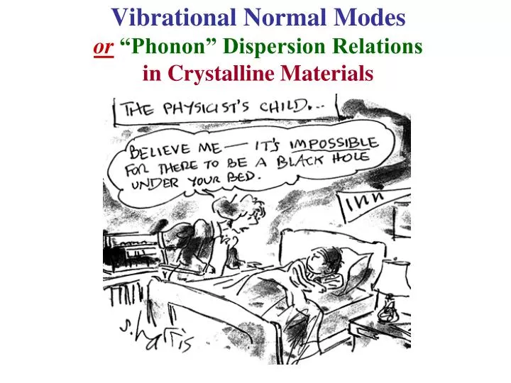
Vibrational Normal Modes or “Phonon” Dispersion Relations in Crystalline Materials. “Phonon” Dispersion Relations in Crystalline Materials. So far, we’ve discussed results for the “ Phonon ” Dispersion Relations ω(k) (or ω(q) ) only in model, 1-dimensional lattices.

E N D
Vibrational Normal Modesor“Phonon” Dispersion Relationsin Crystalline Materials
“Phonon” Dispersion Relationsin Crystalline Materials • So far, we’ve discussed results for the “Phonon” Dispersion Relationsω(k) (or ω(q)) only in model, 1-dimensional lattices. • Now, we’ll have a Brief Overview of the Phonon Dispersion Relationsω(k) in real materials. • Both experimental results & some of the past theoretical approaches to obtaining predictions of ω(k) will be discussed. • As we’ll see, some past “theories” were quite complicated in the sense that they contained N (N >> 1) parameters which were adjusted to fit experimental data. So, (my opinion) They were really models & NOT true theories. • As already mentioned, the modern approach is to solve the electronic problem first, then calculate the force constants for the lattice vibrational predictions by taking 2nd derivatives of the total electronic ground state energy with respect to the atomic positions.
Two Part Discussion Part I • This will be a general discussion of ω(k) in crystalline solids, followed by the presentation of some representative experimental results for ω(k) (obtained mainly in neutron scattering experiments) for several materials. Part II • This will be a brief survey of variousLattice Dynamics models, which were used in the past to try to understand the experimental results. • As we’ll see, some of these models were quite complicatedin the sense that they contained LARGE NUMBERSof adjustable parameters which were fit to experimental data. • The modern method is to first solve the electronic problem. Then, the force constants which for the vibrational problem are calculated by taking various 2nd derivatives of the electronic ground state energy with respect to various atomic displacements.
The Classical Vibrational Normal Mode Problem (in the Harmonic Approximation) ALWAYS reduces to solving: Here, D(q) ≡ The Dynamical Matrix D(q) ≡ The spatial Fourier Transform of the “Force Constant” Matrix Φ q ≡ wave vector, I ≡identity matrix ω2≡ ω2(q) ≡ vibrational mode eigenvalue
NOTE! • There are, in general, 2 distinct types of vibrational waves (2 possible wave polarizations) in solids: Longitudinal • Compressional: The vibrational amplitude is parallel to the wave propagation direction. and Transverse • Shear: The vibrational amplitude is perpendicular to the wave propagation direction. • For each wave vectork, these 2 vibrational polarizations will give 2 different solutionsforω(k).
We also know that there are, at least, 2 distinct branches ofω(k)(2 different functions ω(k) for each k) The Acoustic Branch • This branch received it’s name because it contains long wavelength vibrations of the form ω = vsk, where vs is the velocity of sound. Thus, at long wavelengths, it’s ω vs. k relationship is identical to that for ordinary acoustic (sound) waves in a medium like air. The Optic Branch Discussed on the next page:
The Optic Branch • This branch is always at much higher frequencies than the acoustic branch. So, in real materials, a probe at optical frequencies is needed to excite these modes. • Historically, the term “Optic” came from how these modes were discovered. Consider an ionic crystal in which atom 1 has a positive charge & atom 2 has a negative charge. As we’ve seen, in those modes, these atoms are moving in opposite directions. (So, each unit cell contains an oscillating dipole.) These modes can be excited with optical frequency range electromagnetic radiation. • We’ve already seen that the 2 branches have very different vibrational frequencies ω(k).
So, when discussing the vibrational frequencies ω(k), it is necessary to distinguish between Longitudinal & Transverse Modes(Polarizations) & At the same time to distinguish between Acoustic & Optic Modes. • So, there are four distinct kinds of modes for ω(k). • The terminologies used, with their abbreviations are: Longitudinal Acoustic Modes LA Modes Transverse Acoustic Modes TA Modes Longitudinal Optic Modes LO Modes Transverse Optic Modes TO Modes
A Transverse Acoustic Mode for the Diatomic Chain The type of relative motion illustrated here carries over qualitatively to real three-dimensional crystals. The vibrational amplitude is highly exaggerated! This figure illustrates the case in which the lattice has some ionic character, with + & - charges alternating:
A Transverse Optic Mode for the Diatomic Chain The type of relative motion illustrated here carries over qualitatively to real three-dimensional crystals. The vibrational amplitude is highly exaggerated! This figure illustrates the case in which the lattice has some ionic character, with + & - charges alternating:
Polarization & Group Velocity LA Modes Frequency, TA Modes Wave vector, K 0 (p/a) A crystal with 2 atoms or more per unit cell will ALWAYS have BOTH Acoustic & Optic Modes. If there are n atoms per unit cell in 3 dimensions, there will ALWAYS be 3 Acoustic Modes & 3n -3 Optic Modes. Vibrational Group Velocity: Acoustic Modes Speed of Sound:
Polarization Lattice Constant, a yn-1 xn yn xn+1 TA & TO LA & LO OpticModes For 2 atoms per unit cell in 3 d, there are a total of 6 polarizations The transverse modes (TA & TO) are often doubly degenerate, as has been assumed in this illustration. LO TO Acoustic Modes LA Frequency, TA 0 p/a Wave vector, K
1st Brillouin Zones:For the FCC, BCC, & HCP Lattices Direct: FCC Reciprocal: BCC Direct: BCC Reciprocal: FCC Direct: HCP Reciprocal: HCP (rotated)
1st Brillouin Zone of FCC Lattice Direct LatticeReciprocal Lattice
MeasuredPhonon Dispersion Relations in Si (Inelastic, “Cold” Neutron Scattering) Normal Mode Frequencies(k) Plotted for kalong high symmetry directions in the 1st BZ. 1st BZ for the SiLattice (diamond; FCC, 2 atoms/unit cell) ω k
Normal Modes of Silicon L = Longitudinal, T =Transverse O =Optic, A =Acoustic
Theoretical (?)Phonon Dispersion Relations in GaAs Normal Mode Frequencies(k) Plotted for kalong high symmetry directions in the 1st BZ. 1st BZ for the GaAsLattice (zincblende; FCC, 2 atoms/unit cell) ω k
For Diamond Structure materials, such as Si, & Zincblende Structure materials, such as GaAs, for each wavevector q, there are 6 branches (modes) to the “Phonon Dispersion Relations”ω(q)
For Diamond Structure materials, such as Si, & Zincblende Structure materials, such as GaAs, for each wavevector q, there are 6 branches (modes) to the “Phonon Dispersion Relations”ω(q) • These are:3 Acoustic Branches 1 Longitudinal mode: LA branch or LA mode + 2 Transverse modes:TA branches or TA modes In the acoustic modes, the atoms vibrate in phase with their neighbors.
For Diamond Structure materials, such as Si, & Zincblende Structure materials, such as GaAs, for each wavevector q, there are 6 branches (modes) to the “Phonon Dispersion Relations”ω(q) • These are:3 Acoustic Branches 1 Longitudinal mode: LA branch or LA mode + 2 Transverse modes:TA branches or TA modes In the acoustic modes, the atoms vibrate in phase with their neighbors. and 3 Optic Branches 1 Longitudinal mode: LO branch or LO mode + 2 Transverse modes: TO branches or TO modes In the optic modes, the atoms vibrate out of phase with their neighbors.
MeasuredPhonon Dispersion Relations inFCC Metals (Inelastic, “Cold” Neutron Scattering) Pb 1st BZ for the FCCLattice Cu
MeasuredPhonon Dispersion Relations inFCC Metals (Inelastic X-Ray Scattering) Al Unit Cell for the FCC Lattice 1st BZ for the FCCLattice
Measured Phonon Dispersion Relations for C in the Diamond Structure (Inelastic X-Ray Scattering) 1st BZ for the DiamondLattice
Measured Phonon Dispersion Relations for Ge in the Diamond Structure (Inelastic “Cold” Neutron Scattering) 1st BZ for the DiamondLattice L
MeasuredPhonon Dispersion Relations for KBr in the NaCl Structure (FCC, 1 Na & 1 Cl in each unit cell) (Inelastic, “Cold” Neutron Scattering) 1st BZ for the DiamondLattice L
Measured & CalculatedPhonon Dispersion Relations for Zr in the BCC Structure(Inelastic, “Cold” Neutron Scattering) Data Points, 2 Different Theories: Solid & Dashed Curves) 1st BZ for the BCCLattice
Models for Normal Modes ω(k)in 3 Dimensions Outline of Calculations withNewton’s 2nd Law Equations of Motion Assuming the Harmonic Approximation (r) Interatomic Potential s Displacements from Equilibrium In the harmonic approximation, expandin a Taylor’s series of displacements s aboutthe equilibrium positions.Cut off the series at the term that is quadratic in the displacements. The following illustrates this procedure: nth unit cell N unit cells, each with n atoms means that there are 3Nn Coupled Newton’s 2nd Law Equations of Motion
Lattice Dynamics in 3 Dimensions - Outline Calculations of ω(k) in the Harmonic Approximation (r) Interatomic Potential s Displacements from Equilibrium Expand in a Taylor’s series in displacements s about equilibrium. Keep only up to quadratic terms: nth unit cell Hamiltonian in the Harmonic Approx. “Force Constant” Matrix Analogous to 1 d F = -(d/dx) Resulting Newton’s 2nd LawEquation of Motion N unit cells, each with n atoms means that there are 3Nn Coupled Newton’s 2nd Law Equations of Motion
Force Constant Matrix Properties Analogous to the 1d Harmonic Oscillator Analogous to the 1 d Spring Constant Schematic view of the lattice. Various symmetries of the Force Constant Matrix
Formally Solve the Equations of Motion – Use a Spatial Fourier Series Approach After some work, the equations of motion become:
So, the mathematics of All ofFORMAL Lattice Dynamics can be summarizedas finding solutions to • The remainder is the use of various models & theories for the “force constants” which enter the force constant matrix Ф & thus the dynamical matrix D.
There are many different models & theorieswhich were designed to determine the force constants which enter the dynamical matrix D. These can broadly be divided into 4 groups: 1.Force Constant Models 2.Shell Models 3.Bond Models 4.Bond Charge Models • Within each group, there are MANYvariations on these models! • Going down the list: The models get more complex & (in my opinion) harder to understand in terms of the physics behind them.
Common Features of All Models (or Theories): 1. All model the ion-ion interactions with some parameters in the force constant matrix . 2.All find these parameters by fitting to various experimental quantities. A few of the many quantities used to do the fitting are: Bulk Modulus; Shear Modulus; BZ center LO, TO, LA, & TA frequencies; BZ edge LO, TO, LA, TA frequencie + Many Others Since the goal was to explain neutron scattering data, people tried to use non-neutron scattering data to fit the parameters. 3. All used thefitted parameters in the matrix to compare to neutron scattering data & to predict results of neutron scattering experiments.
Force Constant Models • These models are the crudest approach taken & the closest in spirit & actual calculationsto the 1d models we discussed. • They model the force constant matrix with as few parameters as possible & fit to data mentioned. • Assumption:The atoms (the ion core + valence electrons) are HARD SPHERES, coupled by “springs”, characterized by spring constants (~ like the 1d models) • They include short range forces only. But have no Coulomb forces! • There are various types of “springs”: 1st, 2nd, 3rd, 4th, 5th, … neighbor coupling!! • The spring forces have directional dependences, with different spring constants for coupling in different directions.
The “best” force constant models require 12 to 20DIFFERENTforce constants per material! A Rhetorical Question: Is this physically reasonable & satisfying? • Such models give good (q)for the Group IV covalent solids: C (diamond), Si, Ge, α-Sn • But, they FAIL for many covalent & ionic compounds, such as The III-V & II-VI materials, GaAs, CdTe, etc. • This happens because Coulomb (ionic) forces are ignored! • Also, the bonds in these compounds are partially ionic (there is a charge separation).
A Rhetorical Question!! Is a 15 to 20 adjustable parameter “theory” REALLY A THEORY? • A quote in several references: “The parameters are not easily understood from a physical point of view.” (In my opinion, this is putting it mildly!) • Often, these models need up to 5th & 6th neighbor (or higher) force constants!
A physically realistic qualitative expectation for relative size of the force constants connecting neighbors at various distances is: The force constant size should decrease as the distance increases. • However, it’s been found that, in order to get a good fit to data, some of these models require instead that the size of some force constants must increase with increasing distance!! For example: Φ4nn > Φ1nn & other, absurd, completely unphysical results!
In addition, no matter how many force constants are assumed, these models cannot explain a lot of data! • For example, the flattening of TAnear the BZ edges. • Often, these models were found to work ok for purely covalent solids like C (diamond), Si, Ge,… but to do a poor job on ionic compounds in which Coulomb Effects are important! • To deal with these problems, “better” theories or models were introduced. One such group of models is called The Shell Models
Shell Models • The force constant models all assume “hard sphere” atoms(ion core + valence electrons). From our discussion of bonding & from electronic properties studies, we know that this is a Very BAD assumption for covalently bonded solids as well as for many other solid types! • Our knowledge of bonding & electronic properties tells that: The valence electrons are NOTrigidly attached to the ions! The Main Idea of the Shell Model: Each atom is modeled as a rigid ion core plus an “independent” valence electron shell. Also, the valence electron shell AND the ion core can move. That is, the Atoms are Deformable!
So, in the extensions of the force constant models to the Shell Models, the atoms are deformable! That is, The ions & valence electron shells are all moving. • Also, Coulomb Interactions are included by putting charges on the shells & the ion cores. • In these models, the atomic displacements induce dipole moments on the atoms. So, there are dipole-dipole interactions between unit cells as well as force constants to couple the cells.
Best Shell Model results for (q) • Ge -A good fit to neutron data is found with only 5 parameters! • GaAs & other Compounds - A good fit to neutron data is found with ~ 10 - 12 parameters. • That is, the combined force constant shell model doesn’t do much better than pure force constant models! Physics Criticisms 1. The valence electrons in covalent materials are NOT in the shells around the ion cores! 2. The valence electrons in these materials ARE in the covalent bonds between the cores! 3. The fitting parameters are ~unphysical & have limited use for modeling properties other than (q).
Other Physics Criticisms • These models make an artificial divisionof valence electrons between atoms which are covalently bonded together. • Actually, these valence electrons are shared in the covalent bonds! • So, people introduced “better” theories or models, such as the Bond Models.
Bond Models • In covalent materials, the valence electrons are in the covalent bonds between the atoms & along the directions from an atom’s near neighbors. • Bond models: Extend the “Valence Force Field” Method to covalent solids. • Valence Force Field Method (VFFM): • Used in theoretical molecular chemistry to explain vibrational properties of covalent molecules. • In this model, the vibrations are analyzed in terms of “valence forces” for bond stretching & bending.
VFFM Advantages: • The force constants for bond stretching & bending are ~ characteristic of particular bonds & are transferable from one molecule to another, which contains same bond (e.g. the force constants for a C-C bond are ~ the same no matter what solid it is in! Bond Models: • The force constants are ~ the same for an A-B bond in a solid as they are in molecules.
Extension of the VFFM to covalent solids, 2 atoms / unit cell. • The bond potential energy V is expanded about equilibrium positions for all possible degrees of freedom of bending, stretching, etc. of bond. • Expansion stopped at 2nd order in deviations from equilibrium. Simple harmonic oscillators in all degrees of vibrational freedom!
Disappointment! • Despite the greater physical appeal & (hopefully) the better physical realism of such models, to get good fits to ω(q)(neutron scattering data), the bond models need ~ a similar number of parameters as the shell models! So, after all the work on the Bond Models, it turns out that there is no real advantage of them over the shell models!
The Keating Model ≡ The VFFM with 2 or 3 parameters + a charge parameter. • Good for elastic properties at long wavelengths (later). • BAD for frequencies! Other models & extensions of the VFFM: 5 or 6 parameters • Often do well for trends in frequencies & BAD for other vibrational properties (like elastic properties)! • So, people introduced “better” theories (models) like the Bond Charge Models
Bond Charge Models • The most difficult part of modeling the force constant matrix is accurately including the long-range (Coulomb) electron-ion interaction. • The Shell Models + charges: Attempts to simulate this. However, fails to account for dielectric screening. Also, for covalent bonds, charge is not on atoms, but between them! • The Bond Models: Account for covalent bonding, but neglects Coulomb screening.
Review of Screening: • Look at a specific ion at origin. • Let the Coulomb interaction with one electron Vo(r). • But, the presence of other electrons reduces this: • The presence of all other charges (ions & electrons) near ion of interest causes effective interaction to be reduced. • It is shown in EM courses that the true potential is of form V(r) Vo(r)exp(-r/ro) • Usually, this is simulated in simpler way: V(r) Vo(r)/ε Here, ε =dielectric constant
Screening in classical E&M: V(r) Vo(r)/ε ε = dielectric constant: Really, ε = ε(q,ω) but neglect this. • This is too simple to work well for vibrational spectra! Reason: the implicit assumption is that valence electrons are “free” , except for Coulomb interactions with ion of interest. • We could treat Coulomb effects (ion with charge Ze) by V(r) -(Ze2)/(εr), but this is too crude. • Instead, localize some of valence electrons on the bonds, so that some screen in this way & others don’t.