Ch1. Fundamentals of Computer Design 1. Formulas

1. ECE Department University of Massachusetts Dartmouth285 Old Westport Rd.North Dartmouth, MA 02747-2300 Ch1. Fundamentals of Computer Design 1. Formulas ECE562 Advanced Computer Architecture Prof. Honggang Wang Slides based on the PowerPoint Presentations created by David Patterson as part of the Instructor Resources for the textbook by Hennessy & Patterson Updated by Honggang Wang.

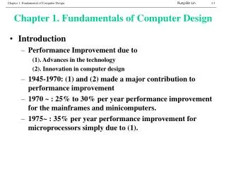
2. Outline • Technology Trends • Careful, quantitative comparisons: Formulas • Define and quantify power • Define and quantify relative cost • Define and quantify dependability

3. Moore’s Law: 2X transistors / “year” • “Cramming More Components onto Integrated Circuits” • Gordon Moore, Electronics, 1965 • # on transistors / cost-effective integrated circuit double every N months (12 ≤ N ≤ 24)

4. Technology Performance Trends • Drill down into 4 technologies: • Disks, • Memory, • Network, • Processors • Compare ~1980 Archaic vs. ~2000 Modern • Performance Milestones in each technology • Bandwidth vs. Latency improvements in performance over time • Bandwidth: number of events per unit time • E.g., M bits / second over network, M bytes / second from disk • Latency: elapsed time for a single event • E.g., one-way network delay in microseconds, average disk access time in milliseconds

5. Disks: Archaic v. Modern CDC Wren I, 1983 (Sunstar) • 3600 RPM • 0.03 GBytes capacity • Tracks/Inch: 800 • Bits/Inch: 9550 • Three 5.25” platters • Bandwidth: 0.6 MBytes/sec • Latency: 48.3 ms • Cache: none Seagate 373453, 2003 • 15000 RPM (4X) • 73.4 GBytes (2500X) • Tracks/Inch: 64000 (80X) • Bits/Inch: 533,000 (60X) • Four 2.5” platters (in 3.5” form factor) • Bandwidth: 86 MBytes/sec (140X) • Latency: 5.7 ms (8X) • Cache: 8 MBytes

6. Latency Lags Bandwidth (for last ~20 years) • Performance Milestones • Disk: 3600, 5400, 7200, 10000, 15000 RPM (8x, 143x) (latency = simple operation w/o contention BW = best-case)

7. Memory Archaic • 1980 DRAM(asynchronous) • 0.06 Mbits/chip • 16-bit data bus per module, 16 pins/chip • 13 Mbytes/sec • Latency: 225 ns • (no block transfer) Modern • 2000Double Data Rate Synchr. (clocked) DRAM • 256.00 Mbits/chip (4000X) • 64-bit data bus per DIMM, 66 pins/chip (4X) • 1600 Mbytes/sec (120X) • Latency: 52 ns (4X) • Block transfers (page mode)

8. Latency Lags Bandwidth (last ~20 years) • Performance Milestones • Memory Module: 16bit plain DRAM, Page Mode DRAM, 32b, 64b, SDRAM, DDR SDRAM (4x,120x) • Disk:3600, 5400, 7200, 10000, 15000 RPM (8x, 143x) (latency = simple operation w/o contention BW = best-case)

9. "Cat 5" is 4 twisted pairs in bundle Twisted Pair: Copper, 1mm thick, twisted to avoid antenna effect LANs: Archaic v. Modern • Modern • Ethernet 802.3ae • Year of Standard: 2003 • 10,000 Mbits/s (1000X)link speed • Latency: 190 msec (15X) • Switched media • Category 5 copper wire Archaic • Ethernet 802.3 • Year of Standard: 1978 • 10 Mbits/s link speed • Latency: 3000 msec • Shared media • Coaxial cable Coaxial Cable: Plastic Covering Braided outer conductor Insulator Copper core

10. Latency Lags Bandwidth (last ~20 years) • Performance Milestones • Ethernet: 10Mb, 100Mb, 1000Mb, 10000 Mb/s (16x,1000x) • Memory Module:16bit plain DRAM, Page Mode DRAM, 32b, 64b, SDRAM, DDR SDRAM (4x,120x) • Disk:3600, 5400, 7200, 10000, 15000 RPM (8x, 143x) (latency = simple operation w/o contention BW = best-case)

11. CPUs Archaic • 1982 Intel 80286 • 12.5 MHz • 2 MIPS (peak) • Latency 320 ns • 16-bit data bus, 68 pins • Microcode interpreter, separate FPU chip • (no caches) Modern • 2001 Intel Pentium 4 • 1500MHz (120X) • 4500 MIPS (peak) (2250X) • Latency 15 ns (20X) • 64-bit data bus, 423 pins • 3-way superscalar,Dynamic translate to RISC, Superpipelined (22 stage),Out-of-Order execution • On-chip 8KB Data caches, 96KB Instr. Trace cache, 256KB L2 cache

12. CPU high, Memory low(“Memory Wall”) Latency Lags Bandwidth (last ~20 years) • Performance Milestones • Processor: ‘286, ‘386, ‘486, Pentium, Pentium Pro, Pentium 4 (21x,2250x) • Ethernet: 10Mb, 100Mb, 1000Mb, 10000 Mb/s (16x,1000x) • Memory Module: 16bit plain DRAM, Page Mode DRAM, 32b, 64b, SDRAM, DDR SDRAM (4x,120x) • Disk : 3600, 5400, 7200, 10000, 15000 RPM (8x, 143x)

13. Rule of Thumb for Latency Lagging BW • In the time that bandwidth doubles, latency improves by no more than a factor of 1.2 to 1.4 • Stated alternatively: Bandwidth improves by more than the square of the improvement in Latency

14. 6 Reasons for LatencyLags Bandwidth 1. Moore’s Law helps BW more than latency • Faster transistors, more transistors, more pins help Bandwidth • MPU Transistors: 0.130 vs. 42 M xtors (300X) • DRAM Transistors: 0.064 vs. 256 M xtors (4000X) • MPU Pins: 68 vs. 423 pins (6X) • DRAM Pins: 16 vs. 66 pins (4X) • Smaller, faster transistors but communicate over (relatively) longer lines: latency • Feature size: 1.5 to 3 vs. 0.18 micron (8X,17X) • MPU Die Size: 35 vs. 204 mm2 (ratio sqrt  2X) • DRAM Die Size: 47 vs. 217 mm2 (ratio sqrt  2X)

15. 6 Reasons for LatencyLags Bandwidth 2. Distance limits latency improvement • Size of DRAM block long bit and word lines  Increase DRAM access time 3.Bandwidth easier to sell (“bigger=better”) • E.g., 10 Gbits/s Ethernet (“10 Gig”) vs. 10 msec latency Ethernet • 4400 MB/s DIMM (“PC4400”) vs. 50 ns latency • Even if just marketing, customers now trained • Since bandwidth sells, more resources are thrown at bandwidth, which further tips the balance

16. 6 Reasons for LatencyLags Bandwidth 4. Latency helps BW, but not vice versa • Spinning disk faster improves both bandwidth and rotational latency • 3600 RPM  15000 RPM = 4.2X • Average rotational latency: 8.3 ms  2.0 ms • Things being equal, also helps BW by 4.2X • Lower DRAM latency More access/second (higher bandwidth) • Higher linear density helps disk BW (and capacity), but not disk Latency

17. 6 Reasons LatencyLags Bandwidth (cont’d) 5. Bandwidth hurts latency • Queues help Bandwidth, hurt Latency (Queuing Theory) • Adding chips to widen a memory module increases Bandwidth but higher fan-out on address lines may increase Latency 6. Operating System overhead hurts Latency more than Bandwidth • Long messages amortize overhead; overhead bigger part of short messages

18. Summary of Technology Trends • For disk, LAN, memory, and microprocessor, bandwidth improves by square of latency improvement • In the time that bandwidth doubles, latency improves by no more than 1.2X to 1.4X • Lags probably are even larger in real systems, as bandwidth gains multiplied by replicated components • Multiple processors in a cluster or even in a chip • Multiple disks in a disk array • Multiple memory modules in a large memory • Simultaneous communication in switched LAN • HW and SW developers should innovate assuming Latency Lags Bandwidth • If everything improves at the same rate, then nothing really changes • When rates vary, require real innovation

19. Outline • Review • Technology Trends: • Careful, quantitative comparisons: Formulas • Define and quantify power • Define and quantify relative cost • Define and quantify dependability

20. Define and quantify power ( 1 / 2) • For CMOS chips, traditional dominant energy consumption has been in switching transistors, called dynamic power • For mobile devices, energy metric better • For a fixed task, slowing clock rate (frequency switched) reduces power, but not energy • Capacitive load a function of number of transistors connected to output and technology, which determines capacitance of wires and transistors • Dropping voltage helps both, e.g., dropped from 5V to 1V • To save energy & dynamic power, most CPUs now turn off clock of inactive modules

21. Example of quantifying power • Suppose 15% reduction in voltage results in a 15% reduction in frequency. What is impact on dynamic power?

22. Define and quantity power (2 / 2) • Because leakage current flows even when a transistor is off, now static power important too • Leakage current increases in processors with smaller transistor sizes • Increasing the number of transistors increases power even if they are turned off • In 2006, goal for leakage is 25% of total power consumption; high performance designs at 40% • Very low power systems even gate voltage to inactive modules to control loss due to leakage

23. Outline • Review • Technology Trends: Culture of tracking, anticipating and exploiting advances in technology • Careful, quantitative comparisons: Formulas • Define and quantity power • Define and quantity relative cost • Define and quantity dependability

24. Define and quantify relative cost Critical Question: What is the fraction of good dies on a wafer (Die Yield)? Assume the wafer yield is 100%: where parameter  corresponds roughly to the # of critical masking levels, a measure of manufacturing complexity estimated at 4.0 for multilevel metal CMOS processes in 2006. To understand the cost of computers, must understand the cost of IC: where 1. Cost of die = Cost of wafer / (Dies per wafer x Die Yield) 2. Testing cost 3. Packaging cost

25. Define and quantify relative cost (cont) Example: Find the die yield for dies that are 1.5 cm on a side and 1.0cm on a side, assuming a defect density of 0.4 per cm-squared and  is 4. Answer: • For larger die: • For smaller die: substitute 2.25 with 1.00

26. Outline • Review • Technology Trends: Culture of tracking, anticipating and exploiting advances in technology • Careful, quantitative comparisons: Formulas • Define and quantity power • Define and quantity relative cost • Define and quantity dependability

27. Define and quantify dependability (1/3) • How decide when a system is operating properly? • Infrastructure providers now offer Service Level Agreements (SLA) to guarantee that their networking or power service would be dependable • Systems alternate between 2 states of service with respect to an SLA: • Service accomplishment, where the service is delivered as specified in SLA • Service interruption, where the delivered service is different from the SLA • Failure = transition from state 1 to state 2 • Restoration = transition from state 2 to state 1

28. Define and quantity dependability (2/3) • Module reliability = measure of continuous service accomplishment (or time to failure). 2 metrics • Mean Time To Failure (MTTF) measures Reliability • Failures In Time (FIT) = 1/MTTF, the rate of failures • Traditionally reported as failures per billion hours of operation • Mean Time To Repair (MTTR) measures Service Interruption • Mean Time Between Failures (MTBF) = MTTF+MTTR • Module availability measures service as alternate between the 2 states of accomplishment and interruption (number between 0 and 1, e.g. 0.9) • Module availability = MTTF / ( MTTF + MTTR)

29. Example calculating reliability • If modules have exponentially distributed lifetimes (age of module does not affect probability of failure), overall failure rate is the sum of failure rates of the modules • Calculate FIT and MTTF for 10 disks (1M hour MTTF per disk), 1 disk controller (0.5M hour MTTF), and 1 power supply (0.2M hour MTTF):

30. Outline • Review • Technology Trends: Culture of tracking, anticipating and exploiting advances in technology • Careful, quantitative comparisons: Formulas • Define and quantity power • Define and quantity relative cost • Define and quantity dependability

31. Summary • Expect Bandwidth in disks, DRAM, network, and processors to improve by at least as much as the square of the improvement in Latency • Quantify Cost (vs. Price) • IC  f(Area2) + Learning curve, volume, commodity, margins • Quantify dynamic and static power • Capacitance x Voltage2 x frequency, Energy vs. power • Quantify dependability • Reliability (MTTF vs. FIT), Availability (MTTF/(MTTF+MTTR)

32. Appendix

33. Disk Concept • A platter from a 5.25" hard disk, with 20 concentric tracks drawnover the surface. Each track is divided into 16 imaginary sectors

34. Example of quantifying power • Suppose 15% reduction in voltage results in a 15% reduction in frequency. What is impact on dynamic power?