Download
1 / 40
470 likes | 765 Vues
Earthquake Prediction and Forecasting. “The Holy Grail of Seismology”.

E N D
Earthquake Prediction and Forecasting “The Holy Grail of Seismology”
In recent years, a popular notion has taken root in the minds of many southern Californians: large earthquakes always happen in the morning! The magnitude 7.3 Landers earthquake and its largest aftershock, the Big Bear earthquake, shook awake a lot of people in 1992. Those events were still fresh on their minds when another large rupture, the magnitude 6.7 Northridge earthquake disturbed the sleep of millions in and around the Los Angeles area. Most recently, the Hector Mine earthquake of October 1999 struck at 2:47 am. Never mind that the Joshua Tree earthquake, which ultimately led to the Landers rupture two months later, struck just before 10:00 pm Pacific Daylight Time; a pattern was perceived independently by countless residents, especially those who could remember that the 1987 Whittier Narrows occurred just before 8:00 am. When this "discovery" was brought up over lunch or coffee with others who'd noticed the same thing, that only served to reinforce it. Now it is part of the "earthquake culture" in this area.
The question then becomes “Can earthquakes be predicted?” The answer is probably not, based on our current state of knowledge. A variety of prediction methods have been used for centuries, ranging from accounts of “earthquake weather” and the time of day, to the alignment of planets and jumpiness of animals, none of which are accepted. • In general, for a prognostication to be referred to as a viable prediction it must include: • 1. Fault that will rupture • 2. Magnitude of earthquake • 3. Date (or date range) of earthquake
Hai'cheng and Tangshan • A successful prediction of a major earthquake in Hai'cheng, China in 1975 was hailed as the beginning of earthquake prediction worldwide. Abnormal behavior in domestic and wild animals led the administration to issue a warning that a large earthquake was about to hit. But what is often not told, is that preceding the main shock, came dozens of small foreshocks that shook Hai'cheng and the neighboring areas frightening most of the people enough to camp out in the open. This is what saved lives, not the prediction. A year later in 1976 similar animal precursors were observed at Tangshan, another Chinese city, but there were no foreshocks and so no prediction was issued. Close to 655,000 people were killed at Tangshan in a major quake and earthquake prediction was back to square one. Strange animal behavior cannot be ruled out altogether. But how does one differentiate between a genuine precursor and one that isn't. It is still not know to clearly what the animals sense, that scientific instruments cannot.
Damage to school resulting from the 1976 Tangshan earthquake Damage to water main due to fault rupture Damage to railroad building
The New Madrid Earthquake Prediction of 1990 • In the fall of 1989, Dr. Iben Browning predicted that an earthquake similar in both size and extent to those which struck the area in 1811-1812 would strike the region on December 3rd, 1990, give or take 48 hours. His forecast was based on a 179-year cycle of tidal forces of the Sun and moon that produce stress on the Earth. Such forces were last felt in 1811. The New Madrid Seismic Zone, earthquake epicenters 1980-1990.
Dr. Browning, a climatologist, had been known to have predicted the 1989 Loma Prieta Earthquake a week in advance in an appearance before about 500 business executives and their wives at a convention. He also reportedly predicted the eruption of Mt. St. Helens in 1980. Collapse of the Cypress structure, Loma Prieta earthquake, 1989. Eruption of Mt. St. Helens, 1980.
The prediction was so specific and apocalyptic, it provoked near hysteria throughout the region. The media leaped on the prediction and suddenly the populace became all too aware of the threat. Schools and factories in the region closed and groups such as the Red Cross wasted precious funds in their efforts to calm the public. Unfortunately, Dr. Browning’s prediction was scientifically groundless, and did not occur.
The ultimate responsibility for the misleading quake prediction has to rest with Browning and the scientific community. Scientists had the ultimate responsibility to call Browning a “quack” early on, yet wanted no part of Browning or his prognostications.
The 2004 Southern California Prediction • More recently, in 2004, an international research tema led by Dr. Vladimir Keilis-Borok, a UCLA seismologist, predicted that a magnitude 6.5 earthquake would strike the southern California area by September 5th of that year. Dr. Vladimir Keilis-Borok
Keilis-Borok, a seismologist and mathematical geophysicist thought he and his team had found that a precursory chain of small quakes that had occurred in the past and would lead to future larger earthquakes. Based on this method, the team had correctly predicted the Dec. 22, 2003 magnitude 6.5 Paso Robles earthquake, as well as an 8.1 quake in 2003 off Japan’s Hokkaido island. The region of southern California in which Keilis-Borok predicted the earthquake would hit
In the vicinity of a long chain of small earthquakes, the seismologists looked back and see the areas history over the preceding years. If the area had a certain pattern of seismicity, a nine-month alarm is released for the area of concern. • By September 6th, seismologists had realized that this was just one more in a long line of prediction methods that haven’t worked reliably.
In 1976, the National Academy of Sciences published a list of suggested physical clues for earthquake prediction. These include changes in seismic P-wave velocity, ground uplift and tilt, radon emission, electrical resistivity, and the number of local earthquakes.
Unfortunately, as we have seen, predictions using these techniques usually do not “pan out”. Instead, long-term earthquake forecasts are made by studying paleoseismology. Paleoseismology is the study of the ancient earthquake record through fossil earthquakes. Several methods of this have been tried including the uplift of seashores produced by sudden fault slip, and measurement of growth rings in large trees whose root systems often cross the fault. More precise methods are now in place that can track sequences of great earthquakes by examining trenches across the fault. Tracing rock layers within a trench across the Hayward Fault Trenching across the Hayward Fault, northern California
Trenching usually takes place in faults near releasing bends. These releasing bends are generally swamps or marshes. During strong shaking of the ground during an earthquake, water-saturated sand layers beneath the surface may become liquefied. The weight of the overlying rocks and soil above then causes the water and sand to rise to the surface, forming a layer of sand called blows, boils or volcanoes. These sand layers may cover any organic material in the area, turning it over time into peat, which can be dated using C14 age dating techniques. Following this, the area may return to a marshy condition, until the next earthquake, when the cycle repeats. Peat layers offset by San Andreas at Pallet Creek site
16-foot excavation along the San Andreas Fault near Pallet Creek. Kerry Sieh has dated these peat layers to determine the dates of past earthquakes.
Black strata are peat layers, datable by 14C methods, that show increasing amounts of vertical displacement with depth, owing to cumulative slip from repeated earthquakes. Vertical component of displacement visible here is a few percent of net displacement, which is chiefly strike slip, approximately normal to trench wall, with block on right moving toward observer. Uppermost, unfaulted deposits postdate 1857 earthquake; lowermost peat bed on southwest side of fault was deposited about A.D. 800. Modified from Sieh (1978). San Andreas fault exposed in southeast wall of 2a trench at Pallett Creek, Calif., 55 km northeast of Los Angeles.
Previous San Andreas fault ruptures at Pallett Creek (Mojave section) Preferred Event Date Possible Date Range Years Until Next Event January 9, 1857 January 9, 1857 greater than 147 December 8, 1812 December 8, 1812 44.08 1480 A.D. 1465 - 1495 A.D. 332 1346 A.D. 1329 - 1363 A.D. 134 1100 A.D. 1035 - 1165 A.D. 246 1048 A.D. 1015 - 1081 A.D. 52 997 A.D. 981 - 1013 A.D. 52 797 A.D. 775 - 819 A.D. 200 734 A.D. 721 - 747 A.D. 63 671 A.D. 658 - 684 A.D. 63 before 529 A.D. ??? - 529 A.D. greater than 142 Based on the above data, it suggests the San Andreas ruptures with a large magnitude earthquake (Mag. 8.0+) every 145 years, on the average. But there is a large variation. The greatest time interval was over 300 years and the smallest as short as 52 years.
Wallace Creek • A number of little gullies cross the San Andreas Fault along the Carrizo Plain. These gullies used to flow straight across the fault, but now are offset by the strike-slip motion of the fault. For example, Wallace Creek, is offset 420 feet (130 meters) across the fault. Sediments deposited in the channel of Wallace Creek prior to its offset are 3,700 years old based on C14 age dating. The rate of slip is the amount of the offset – 130 meters – divided by the age of the channel which is offset – 3,700 years – 3.5 cm (slightly less than 1 ½ inches) per year. San Andreas Fault
During the great Fort Tejon Earthquake of 1857 the channel was offset as much as 9 to 12 meters. How long would it take for the fault to build up as much strain as it released in 1857? To find out, divide the 1857 slip – 9 to 12 meters – by the slip rate 3.5 cm/yr – to get 257 to 342 years, an estimate of the recurrence interval for this part of the fault. Paleoseismic studies indicate that the last earthquake to strike this part of the fault prior to 1857 was around the year 1480, an interval of 370 to 380 years, which agrees with our calculations. Based on our lowest estimate of 257 years, we really shouldn’t expect this section of the San Andreas to rupture until after the year 2100. Geologic map showing relationships observed in previous photos
The Parkfield Experiment • The seismographic record in California has established that moderate-sized earthquakes (ML 5.5 to 6) have occurred near the town of Parkfield, located in the central portion of the state in 1901, 1922, 1934 and 1966. There is also evidence from felt reports of similar earthquakes in 1857 and 1881.
Simple subtraction suggests a pattern, with an almost constant recurrence time of about 22 years. If this pattern repeated, another Parkfield earthquake could have been expected about 1988. As a result, a prediction experiment was undertaken here, with placement of ultra-sensitive seismographs in order to measure any possible ground motion prior to the quake. Surface fault motions were monitored continuously by creep meters, and geodetic surveys began with special laser geodimeters that measure the distance across the fault between points. Anything that could be used as a reproducable precursor to an impending large earthquake. Laser geodimeter measures changes in distance across the San Andreas Fault near Parkfield. Changes in distances may indicate a precursor to an upcoming earthquake.
A geodolite shown herecan measure changes in distance across a fault zone very accurately. Small changes in atmospheric conditions could cause variations in measurement, so a plane is employed to account for factors such as humidity and airborne particles. • If changes in distance between points are detected, this could indicate a rapid buildup in strain along the fault and signal an impending quake.
The San Andreas fault in central California. A "creeping" section (green) separates locked stretches north of San Juan Bautista and South of Cholame. The Parkfield section (red) is a transition zone between the creeping and southern locked section. Stippled area marks the surface rupture in the 1857 Fort Tejon earthquake.
Significant earthquakes have occurred on the Parkfield section of the San Andreas fault at fairly regular intervals - in 1857, 1881, 1901, 1922, 1934 and 1966. The next significant earthquake was anticipated to take place within the time frame 1988 to 1993.
The similarity of waveforms recorded in the 1922, 1934 and 1966 events, shown below, is possible only if the ruptured area of the fault is virtually the same for all three events. • Recordings of the east-west component of motion made by Galitzin instruments at DeBilt, the Netherlands. Recordings from the 1922 earthquake (shown in black) and the 1934 and 1966 events at Parkfield (shown in red) are strikingly similar, suggesting virtually identical ruptures.
Parkfield earthquake - Fulfillment of the forecast • The earthquake forecast for the Parkfield section of the San Andreas fault was fulfilled on 9/28/2004 with the Mw 6.0 earthquake at 10:17AM PDT.
Preliminary analysis of the 2004 Parkfield shows that it is dissimilar in some respects to the earlier quakes. The 2004 quake nucleated in the south and ruptured to the north. Unlike the 1934 and 1966 quakes, the 2004 quake was not immediately preceded (by 17 minutes, respectively) by a M4.5 foreshocks. Finally, the 38-year interval between the 1966 and 2004 earthquakes was the longest observed interval in the entire 147 year interval. However, the forecast of the place, magnitude, sense of slip, and rupture endpoints and likelihood of rupture was correct. This bolsters confidence in similar hazard forecasts for the Los Angeles and San Francisco Bay regions. Moreover, the 2001 forecast was based on analysis of geophysical data, published research, and fundamental physical principles. The 2004 quake demonstrates the validity to this approach and the value of collecting data that bears on the earthquake problem. However, accurately forecasting the time of damaging earthquakes remains as a significant challenge. Bridge across San Andreas Fault damaged by the magnitude 6.0 earthquake on September 28, 2004.
Forecasting earthquakes • Forecasting is not prediction • less precise • based upon analysis of earthquake return periods rather than identification of pre-cursor y signs • Active faults or fault segments do not rupture in a random manner • they have characteristic return periods (or at least return period envelopes) • these reflect strain accumulation along the fault and the capacity of the fault to resist strain up to a given characteristic point - for that fault or fault segment • There are complications: • Rupture will not occur according to a rigid timetable - there is a return period envelope rather than specific date • Strain may be released by one large quake or a number of smaller ones (e.g. Marmara Sea south of Istanbul) • this has implications for risk assessment
San Andreas example • Prior to 1906 M 8.25 San Francisco quake ~ 3.2m displacement across fault in 50 years • Post-quake rebound on the fault was ~ 6.5m • Amount of time for strain released in quake to accumulate • (6.5/3.2) x 50 ~100 y • Return period until next comparable quake = 100y • Assumes • uniform strain accumulation • quake did not alter • fault properties
Problems with forecasting • Forecasts only as good as the available catalogues • Historical catalogues good for well studied regions such as California, Japan, Europe, China • Poor for regions of low frequency-high magnitude seismicity • Cascadia subduction zone • New Madrid • Jamaica • Western Europe • Catalogues need to go back further; requires geological studies Cascadia subduction zone
The Seismic Gap concept • Defined as an area in an earthquake-prone region where there has been a below average level of seismic energy release • The 1989 Loma Prieta quake filled a gap that had been aseismic since 1906 • Other gaps exist in • Aleutian arc (Alaska) • south of Istanbul • Tokyo • southern California Istanbul seismic gap
Seismic intensity forecasting • Other parameters can be usefully forecast than just timing of a quake • Forecasting seismic intensity at a particular site is vital for: • siting structures such as dams, schools, hospitals & emergency centres • constructing seismic hazard maps • Requires detailed information on geology, ground conditions Seismic intensity forecast map - Tokai (Japan)
Probabilistic forecasting • Most useful way of expressing a forecast of a future quake is in terms of probabilities • Most people are familiar with probabilities as a result of gambling • Example from San Francisco area (Bolt, 1999) • 5 quakes > M = 6.75 in 155 y between 1836 & 1991 • if events are random, another quake of 6.75 can be expected in 155/5 y = 31 y with high probability • Problem: quakes not entirely random. On a particular fault system may be clustered (due to stress transfer) or follow certain trends • Alternative method of probabilistic forecasting is based on the ELASTIC-REBOUND model • Based upon estimates of strain accumulation across fault
Strain measurement and forecasting • Geological mapping undertaken to define active fault segments • Assumption made that a discrete segment will rupture in one go • As Seismic moment links magnitude with rupture length this gives measure of maximum expected earthquake • Relationship between Ms and fault rupture length L: Ms = 6.10 + 0.70 log L
Amount of slip Time Magnitude 6 Calculating probabilities • Next: determine slip history of each segment • Calculate strain accumulation rate for each segment • Slip history for fault segment can then be plotted against time • As slip is related to quake magnitude allows recurrence intervals between quakes greater than a given magnitude to be determined
Quake frequency Recurrence time T2 T2 T1 T1 The quake probability histogram • Construct histogram showing No. of quakes that occur with each specified recurrence time • Most probable recurrence interval is that which divides histogram into two equal areas • If time since last quake in the magnitude range is T1, the probability of the next quake occurring in T1 - T2 years = ratio of red area to yellow area • As recurrence time T2 increases ratio approaches 1 and a quake becomes virtually certain • The more consistent the recurrence time the better the forecast
The quake probability histogram & the San Andreas • Suited to California & San Andreas fault system because active faults exposed at surface • Enables displacements to be measured easily and strain to be monitored • Method crucially depends on constraining well the number of potentially destructive quakes in historic time and their ages • For more discussion of problems see Bolt (1999) p228 - 229)
Predicting earthquakes • A highly controversial issue in seismology • Involves giving a precise warning about the timing and size of a future quake • Reliant upon the occurrence of pre-cursory signs in advance of a quake • Method must be shown to be repeatable in order to be of any use • In a zone of high seismicity, any prediction is going to have greater than chance than zero of being right • On the other hand - a prediction that is not fulfilled ensures that the method is invalid
Proposed earthquake precursors • Changes in seismic velocities • Crustal deformation • Groundwater changes • Gas release • Atmospheric effects • Anomalous animal behaviour • Changes in magnetic and electrical properties of the rocks • the so-called VAN method