Download
1 / 39
390 likes | 404 Vues
Section 9-4 Two Means: Matched Pairs.

E N D
Section 9-4 Two Means: Matched Pairs In this section we deal with dependent samples. In other words, there is some relationship between the two samples so that each value in one sample is paired (naturally matched or coupled) with a corresponding value in the other sample. So the two samples can be treated as matched pairs of values.
Examples: • Blood pressure of patients before they are given medicine and after they take it. • Predicted temperature (by Weather Forecast) and the actual temperature. • Heights of selected people in the morning and their heights by night time. • Test scores of selected students in Calculus-I and their scores in Calculus-II.
First sample: weights of 5 students in April Second sample: their weights in September These weights make 5 matched pairs Third line: differences between April weights and September weights (net change in weight for each student, separately) In our calculations we only use differences d, not the values in the two samples. Example:
n = number of pairs of data. d = mean value of the differences d for the paired sample data (equal to the mean of the x – y values) Notation for Dependent Samples d = individual difference between the two values of a matched pair µd= mean value of the differences d for the population of paired data sd= standard deviation of the differences d for the paired sample data
The sample data are dependent (make matched pairs). Either or both of these conditions is satisfied: The number of pairs of sample data is large (n > 30)or the pairs of values have differences that are from a population that is approximately normal. Requirements
Tests for Matched Pairs The goal is to see whether there is a difference. H0: md= 0 H1: md0, H1: md <0 , H1: md> 0 two tails left tail right tail
d –µd t= sd n degrees of freedom df = n – 1 Hypothesis Test Statistic for Matched Pairs: Note: md=0 according to H0
P-values and Critical Values Use Table A-3 (t-distribution)
Use a 0.05 significance level to test the claim that for the population of students, the meanchange in weight from September to April is 0 kg (so there is no change, on the average) Example:
Weight gained = April weight – Sept. weight d denotes the mean of the “April – Sept.” differences in weight; the claim is d = 0 kg Example: Step 1: claim is d = 0 Step 2: If original claim is not true, we have d ≠ 0 Step 3: H0: d = 0 (original claim)H1: d ≠ 0 Step 4: significance level is = 0.05 Step 5: use the student t distribution
Step 6: find values of d and sddifferences are: –1, –1, 4, –2, 1d = 0.2 and sd= 2.4now compute the test statistic Example: Table A-3: df = n – 1, area in two tails is 0.05, yields a critical value t = ±2.776
Step 7: Because the test statistic does not fall in the critical region, we fail to reject the null hypothesis. Example:
We conclude that there is sufficient evidence to support the claim that for the population of students, the mean change in weight from September to April is equal to 0 kg. Example:
The P-value method: Using technology, we can find the P-value of 0.8605. (Using Table A-3 with the test statistic of t = 0.186and 4 degrees of freedom, we can determine that the P-value is greater than 0.20.) We again fail to reject the null hypothesis, because the P-value is greater than the significance level of = 0.05. Example:
d – E < µd < d + E sd whereE=t/2 n Confidence Intervals for Matched Pairs Critical values of tα/2 : Use Table A-3 with df = n – 1 degrees of freedom.
Construct a 95% confidence interval estimate of d , which is the mean of the “April–September” weight differences of college students in their freshman year. Example: = 0.2, sd = 2.4, n = 5, ta/2 = 2.776 Find the margin of error, E
Construct the confidence interval: Example: We have 95% confidence that the limits of ─2.8 kg and 3.2 kg contain the true value of the mean weight change from September to April.
Dependent samples by TI-83/84 • Enter 1st sample in list L1 and 2nd sample in L2 • Clear screen, type L1─L2→L3 (use STO key) • Press STAT and select TESTS • Scroll down to T-Test for hypotheses testing • or to TInterval for confidence intervals • Select Input: Data (not Stats) and use list L3 • Then proceed as if you had just one sample…
Section 9-5 Comparing Variation in Two Samples
1. The two populations are independent. 2. The two samples are random samples. The two populations are each normally distributed. The last requirement is strict. Requirements
Important: • The first sample must have a larger sample standard deviation s1 than the second sample, i.e. we must have s1 ≥ s2 • If this is not so, i.e. if s1 < s2 , then we will need to switch the indices 1 and 2, i.e. we need to label the second sample (and population) as first, and the first as second.
s1= first (larger) sample st. deviation n1 = size of the first sample s1= st. deviation of the first population Notation for Hypothesis Tests with Two Variances or Standard Deviations s2 n2 s2are used for the second sample and population
Tests for Two Variances The goal is to compare the two population variances (or standard deviations) H0: s1 = s2 H1: s1 s2 , H1: s1> s2 Note: H1: s1< s2 is not considered. Note: no numerical values for s1 or s2 are claimed in the hypotheses. two tails right tail
s1 2 F = s2 2 Test Statistic for Hypothesis Tests with Two Variances Where s12 is the first (larger) of the two sample variances Critical Values:Using Table A-5, we obtain critical F values that are determined by the following three values: 1. The significance level 2. Numerator degrees of freedom = n1 – 1 3. Denominator degrees of freedom = n2 – 1
Values of the F distribution cannot be negative, i.e. F ≥ 0. The exact shape of the F distribution depends on the two different degrees of freedom (numerator df and denominator df) The F distribution is not symmetric. Properties of the F Distribution
If the two populations do have equal variances, then F = will be close to 1 because and are close in value. s1 2 s2 2 s1 s 2 2 2 Use of the F Distribution
If the two populations have radically different variances, then F will be a large number. Remember: the larger sample variance is s1 , so F is either equal to 1 or greater than 1. Use of the F Distribution 2
Consequently, a value of F near 1 will be evidence in favor of the conclusion that 1 = 2 . 2 2 Conclusions from the F Distribution But a large value of Fwill be evidence against the conclusion of equality of the population variances.
To find a critical F value corresponding to a 0.05 significance level, refer to Table A-5 and use the right-tail area of 0.025 or 0.05, depending on the type of test: Finding Critical F Values Two-tailed test: use 0.025 in right tail Right-tailed test: use 0.05 in right tail
Below are sample weights (in g) of quarters made before 1964 and weights of quarters made after 1964. When designing coin vending machines, we must consider the standard deviations of pre-1964 quarters and post-1964 quarters. Use a 0.05 significance level to test the claim that the weights of pre-1964 quarters and the weights of post-1964 quarters are from populations with the same standard deviation. Example:
Example: Step 1: claim of equal standard deviations is equivalent to claim of equal variances Step 2: if the original claim is false, then Step 3: original claim
Step 4: significance level is 0.05 Example: Step 5: involves two population variances, use F distribution variances Step 6: calculate the test statistic For the critical values in this two-tailed test, refer to Table A-5 for the area of 0.025 in the right tail. The critical value is 1.8752.
Example: Step 7: The test statistic F = 1.9729 does fall within the critical region, so we reject the null hypothesis of equal variances. There is sufficient evidence to warrant rejection of the claim of equal standard deviations.
Example: Left tail is not used and need not be shown !
There is sufficient evidence to warrant rejection of the claim that the two standard deviations are equal. The variation among weights of quarters made after 1964 is significantly different from the variation among weights of quarters made before 1964. Conclusion:
Tests about two variances by TI-83/84 • Press STAT and select TESTS • Scroll down to 2-SampFTest press ENTER • Select Input: Data or Stats. For Stats: • Type in sx1:(1st sample st. deviation) • n1:(1st sample size) • sx2:(2nd sample st. deviation) • n2:(2nd sample size) • choose H1:s1 ≠s2 <s2 >s2 • (two tails) (left tail) (right tail)
Tests about two variances (continued) • Press on Calculate • Read the test statistic F=… • and the P-value p=… • Note: the calculator does not require the first sample variance be larger than the second. It can handle both left-tailed and right-tailed tests.