Download
1 / 21
240 likes | 437 Vues
Statistical Power. The ability to find a difference when one really exists. Statistical Power. The probability of rejecting a false null hypothesis (H 0 ). The probability of obtaining a value of t (or z) that is large enough to reject H 0 when H 0 is actually false

E N D
Statistical Power The ability to find a difference when one really exists.
Statistical Power • The probability of rejecting a false null hypothesis (H0). • The probability of obtaining a value of t (or z) that is large enough to reject H0 when H0 is actually false • We always test the null hypothesis against an alternative/research hypothesis • Usually the goal is to reject the null hypothesis in favor of the alternative
Why is Power Important? • As researchers, we put a lot of effort into designing and conducting our research. This effort may be wasted if we do not have sufficient power in our studies to find the effect of interest.
Type I versus Type II Error • A researcher can make two types of error when reporting the results of a statistical test.
Type I Error • The probability of a type I Error is determined by the alpha () level set by the researcher
Type II Error • A type II Error (β) results when the researcher finds that there isn’t a difference, when there really is one.
Statistical Power • Power is the ability of a test to detect a real effect. It is measured as a probability that equals 1 – β.
Power depends on… • To discuss power we need to understand the variables that affect its size. • The alpha level set by the researcher • The sample size (N) • The effect size (e.g., Cohen’s d)
Power and Alpha () • An increase in alpha, say from .05 to .1, artificially increases the power of a study. • Increasing alpha reduces the risk of making a type II error, but increases that of a type I. • Increasing the risk of making a type I error, in many cases, may be worse than making a type II error. • E.g., replacing an effective chemotherapy drug with one that is, in reality, less effective.
Power and Sample Size (N) • Power increases as N increases. • The more independent scores that are measured or collected, the more likely it is that the sample mean represents the true mean. • Prior to a study, researchers rearrange the power calculation to determine how many scores (subjects or N) are needed to achieve a certain level of power (usually 80%).
Power and Effect Size • Effect size is a measure of the difference between the means of two groups of data. • For example, the difference in mean jump ht. between samples of vball and bball players. • As effect size increases, so does power. • For example, if the difference in mean jump ht. was very large, then it would be very likely that a t-test on the two samples would detect that true difference.
A Little More on Effect Size • While a p-value indicates the statistical significance of a test, the effect sizeindicates the “practical” significance. • If the units of measurement are meaningful (e.g., jump height in cm), then the effect size can simply be portrayed as the difference between two means. • If the units of measurement are not meaningful (questionnaire on behaviour), then a standardized method of calculating effect size is useful.
Cohen’s d • Cohen’s d is a common effect size index • It describes the difference between two means in terms of number of standard deviations • The standard deviation (σpooled) represents a weighted average variance from both samples
Hypothetical Example • To understand statistical power the following slides provide a hypothetical example. • Assume that we know the actual effect size. The actual difference between the means.
Jump Height Example • Basketball vs. Volleyball, who jumps higher? • We have 16 athletes in each sample (N=16) • We know the population means are: • Basketball: Mean jump ht = 30 5.7 in. • Volleyball: Mean jump ht = 36 5.7 in. • Alpha = .05 • Using the above information we can graphically demonstrate statistical power. • Knowing there is a difference, how many times out of 100 tests would we be correct?
Step 1. What’s t-critical for the study? • For what t score will we consider there to be a significant difference between bball and vball? • We know, N=32 (df = 30), =.05, and 2-tailed • Use =tinv() in Excel • tinv(.05/2, 30) = 2.36….t critical = 2.36
t critical: -2.36 t-distribution for 30 degrees of freedom / 2 = .025 / 2 = .025 -4 -3 -1 2 4 -2 0 1 3 Use the independent t-test equation For both groups N = 16, Stdev = 5.7 Step 2 t critical: +2.36 We know the mean jump height for bball is 30, then what would vball need to be to get t = 2.36?
t critical: -2.36 t critical: +2.36 t-distribution for 30 degrees of freedom / 2 = .025 / 2 = .025 22 -4 24 -3 28 -1 34 2 4 38 26 -2 30 0 1 32 36 3 Distribution of values ofXV if H0 is true (V = 30) and SEDiff is 2 Critical value ofXV: 34.8 in Step 3 On the actual distribution ofXV,which has a mean of 36, what would be the t-value for 34.8 in? Can you calculate the probability (area) of getting a mean 34.8 if the real mean is 36?...Type 2 Error
t-distribution for 15 degrees of freedom -4 -3 -1 2 4 -2 0 1 3 t = - 0.87 Distribution of values ofXV if V = 36and SEMean is 1.43. Power (1- β) = .80 β = .20 30.3 31.7 34.6 38.9 41.7 33.2 36 37.4 40.3 34.8 Step 4 tdist(t,df,tails) tdist(.87,15,1) = .20
t critical: -2.36 t critical: +2.36 t-distribution for 30 degrees of freedom / 2 = .025 / 2 = .025 -4 22 -3 24 -1 28 34 2 4 38 -2 26 0 30 32 1 36 3 Distribution of values ofX if H0 is true ( = 30) and SEDiff is 2. Critical value ofX: 34.8 in Distribution of values ofXV if V = 36and SEMean is 1.43. Power (1- β) = .80 β = .20 30.3 31.7 34.6 38.9 41.7 33.2 36 37.4 40.3 34.8 Step 4
Power Calculator • http://www.stat.ubc.ca/~rollin/stats/ssize/n2.html