Performance of second-order systems

1. Performance of second-order systems Modern Control Systems Lecture 12

2. Outline • Design specifications & trade-off • Test input signals • Performance of second-order systems to step input • Standard time-domain performance measures for second-order systems • Effects of a third pole and a zero on the second-order system response

3. Design specifications & trade-off Design specifications for control systems are explicit statements in terms of performance measures, which indicate how well the system should perform the task for which it is designed. Trade-off is often necessary to provide a sub-optimal solution in control system design.

4. Test input signals Test input signals are selected and standard input signals, aiming to test the response of a control system. Why test input signals are used? • The actual input signal is unknown. • Good correlation between the response of the system to a test input signal and the system response under normal operating conditions. • Using a standard test input signal allows different designs to be compared. • Many control systems experience input signals similar to test input signals.

5. Test input signals (cont’d) Test input signals commonly used are the step input, the ramp input, and the parabolic input. • Step input derivative of ramp input • Ramp input derivative of parabolic input divided by a scalar • Parabolic input

6. Δ→0 1 e(t) D t D Unit impulse function (Dirac Delta) derivative of unit step The unit impulse δ(t) has useful properties. The response of the system to a unit impulse signal is TF of a system is the Laplace transform of its impulse response.

7. An important property of linear time invariant systems Because of the derivative (or integral) relationship between standard test input signals, the response of linear time-invariant (LTI) systems satisfies: • impulse response = derivative of step response • step response = derivative of ramp response • ramp response = derivative of parabolic response The above property only applies to LTI systems.

8. Example - finding step response the response of the system to a unit step input is Taking the inverse Laplace transform, we have The system response contains two parts – steady-state response & transient response The steady-state response is y(∞)=0.9. The steady-state error is

9. Time response and performance measures The time response of a control system consists of transient response and steady-state response. Time-domain performance specifications/measures are important indices that represent the performance of the control system. The ability to adjust the transient and steady-state responses is a distinct advantage of feedback control systems. Based on the performance measures, system parameters may be adjusted to provide the desired response.

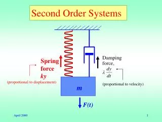
10. Performance of second-order systems to step input Let us consider a typical second-order system to unit step input. The closed-loop output is Rewrite the above equation in standard form The output response is

11. Performance of second-order systems to step input (cont’d) Step response of the second-order system

12. The characteristic equation of The complex conjugate roots Step response of second-order systems As ζ varies with ωn constant, the locus of the closed-loop roots is as shown in the left figure. As ζdecreases, the closed-loop roots approach the imaginary axis, and the output becomes increasingly oscillatory. If ζis increased beyond unity, the response becomes overdamped.

13. Performance of second-order systems to unit impulse input Let us consider the second-order system to unit impulse input. The closed-loop output written in standard form is Impulse response of second-order systems The output response is

14. Closed-loop unit step response: Standard time-domain performance measures for second-order systems (defined in terms of unit step response) • Rise time • Peak time • Percentage overshoot where fv is the final value of the response. For the 2nd-order system under investigation, fv=1 • Settling time. The time for which the response remains within 2% of the final value. where τ is the time constant 1/ζωn.

15. or use to obtain • The swiftness of response (rise time, peak time) • The closeness of the response to the desired response (overshoot, settling time) conflicting requirements To obtain an explicit relation for the peak value and peak time in terms of ζ, we can differentiate impulse response Then Therefore,

16. P.O. and normalised peak time vs ζ for second-order systems P.O. is independent ofωn.

17. For a given ωn, step response is faster for lower ζ. • For a given ζ, step response is faster for larger ωn. ζ=0.2

18. Effects of a third pole on the second-order system response What we have discussed thus far is only for second-order systems in the form of However, the information is useful because many systems possess a dominant pair of roots and the step response can be estimated by the second-order system counterpart. • third-pole For a third-order system with a closed-loop TF its step response can be approximated by the dominant roots of the second-order system if

19. Effects of a zero on the second-order system response • second-order system with one zero The second-order system in the form of has no finite zeros. When adding a zero to the system so that its TF becomes if the location of the zero is relatively near the dominant poles, the zero will materially affect the transient response. without finite zeros with one zero s+a, a/ζωn=A,B,C, or D andζ=0.45