Download
1 / 65
830 likes | 1.75k Vues
Clustering Techniques and Applications to Image Segmentation. Liang Shan shan@cs.unc.edu. Roadmap. Unsupervised learning Clustering categories Clustering algorithms K-means Fuzzy c-means Kernel-based Graph-based Q&A. Unsupervised learning. Definition 1

E N D
Clustering Techniques and Applications to Image Segmentation Liang Shan shan@cs.unc.edu
Roadmap • Unsupervised learning • Clustering categories • Clustering algorithms • K-means • Fuzzy c-means • Kernel-based • Graph-based • Q&A
Unsupervised learning • Definition 1 • Supervised: human effort involved • Unsupervised: no human effort • Definition 2 • Supervised: learning conditional distribution P(Y|X), X: features, Y: classes • Unsupervised: learning distribution P(X), X: features Back Slide credit: Min Zhang
Clustering • What is clustering?
Clustering • Definition • Assignment of a set of observations into subsets so that observations in the same subset are similar in some sense
Clustering • Hard vs. Soft • Hard: same object can only belong to single cluster • Soft: same object can belong to different clusters Slide credit: Min Zhang
Clustering • Hard vs. Soft • Hard: same object can only belong to single cluster • Soft: same object can belong to different clusters • E.g. Gaussian mixture model Slide credit: Min Zhang
Clustering • Flat vs. Hierarchical • Flat: clusters are flat • Hierarchical: clusters form a tree • Agglomerative • Divisive
Hierarchical clustering • Agglomerative (Bottom-up) • Compute all pair-wise pattern-pattern similarity coefficients • Place each of n patterns into a class of its own • Merge the two most similar clusters into one • Replace the two clusters into the new cluster • Re-compute inter-cluster similarity scores w.r.t. the new cluster • Repeat the above step until there are k clusters left (k can be 1) Slide credit: Min Zhang
Hierarchical clustering • Agglomerative (Bottom up)
Hierarchical clustering • Agglomerative (Bottom up) • 1st iteration 1
Hierarchical clustering • Agglomerative (Bottom up) • 2nd iteration 1 2
Hierarchical clustering • Agglomerative (Bottom up) • 3rd iteration 3 1 2
Hierarchical clustering • Agglomerative (Bottom up) • 4th iteration 3 1 2 4
Hierarchical clustering • Agglomerative (Bottom up) • 5th iteration 3 1 2 5 4
Hierarchical clustering • Agglomerative (Bottom up) • Finally k clusters left 3 9 6 1 2 5 8 4 7
Hierarchical clustering • Divisive (Top-down) • Start at the top with all patterns in one cluster • The cluster is split using a flat clustering algorithm • This procedure is applied recursively until each pattern is in its own singleton cluster
Hierarchical clustering • Divisive (Top-down) Slide credit: Min Zhang
Bottom-up vs. Top-down • Which one is more complex? • Which one is more efficient? • Which one is more accurate?
Bottom-up vs. Top-down • Which one is more complex? • Top-down • Because a flat clustering is needed as a “subroutine” • Which one is more efficient? • Which one is more accurate?
Bottom-up vs. Top-down • Which one is more complex? • Which one is more efficient? • Which one is more accurate?
Bottom-up vs. Top-down • Which one is more complex? • Which one is more efficient? • Top-down • For a fixed number of top levels, using an efficient flat algorithm like K-means, divisive algorithms are linear in the number of patterns and clusters • Agglomerative algorithms are least quadratic • Which one is more accurate?
Bottom-up vs. Top-down • Which one is more complex? • Which one is more efficient? • Which one is more accurate?
Bottom-up vs. Top-down • Which one is more complex? • Which one is more efficient? • Which one is more accurate? • Top-down • Bottom-up methods make clustering decisions based on local patterns without initially taking into account the global distribution. These early decisions cannot be undone. • Top-down clustering benefits from complete information about the global distribution when making top-level partitioning decisions. Back
K-means Data set: Clusters: Codebook : Partition matrix: • Minimizes functional: • Iterative algorithm: • Initialize the codebook V with vectors randomly picked from X • Assign each pattern to the nearest cluster • Recalculate partition matrix • Repeat the above two steps until convergence
K-means • Disadvantages • Dependent on initialization
K-means • Disadvantages • Dependent on initialization
K-means • Disadvantages • Dependent on initialization
K-means • Disadvantages • Dependent on initialization • Select random seeds with at least Dmin • Or, run the algorithm many times
K-means • Disadvantages • Dependent on initialization • Sensitive to outliers
K-means • Disadvantages • Dependent on initialization • Sensitive to outliers • Use K-medoids
K-means • Disadvantages • Dependent on initialization • Sensitive to outliers (K-medoids) • Can deal only with clusters with spherical symmetrical point distribution • Kernel trick
K-means • Disadvantages • Dependent on initialization • Sensitive to outliers (K-medoids) • Can deal only with clusters with spherical symmetrical point distribution • Deciding K
Deciding K • Try a couple of K Image: Henry Lin
Deciding K • When k = 1, the objective function is 873.0 Image: Henry Lin
Deciding K • When k = 2, the objective function is 173.1 Image: Henry Lin
Deciding K • When k = 3, the objective function is 133.6 Image: Henry Lin
Deciding K • We can plot objective function values for k=1 to 6 • The abrupt change at k=2 is highly suggestive of two clusters • “knee finding” or “elbow finding” • Note that the results are not always as clear cut as in this toy example Back Image: Henry Lin
Fuzzy C-means Data set: Clusters: Codebook : Partition matrix: K-means: • Soft clustering • Minimize functional • fuzzy partition matrix • fuzzification parameter, usually set to 2
Fuzzy C-means • Minimize subject to
Fuzzy C-means • Minimize subject to • How to solve this constrained optimization problem?
Fuzzy C-means • Minimize subject to • How to solve this constrained optimization problem? • Introduce Lagrangian multipliers
Fuzzy c-means • Introduce Lagrangian multipliers • Iterative optimization • Fix V, optimize w.r.t. U • Fix U, optimize w.r.t. V
Application to image segmentation Original images Segmentations Homogenous intensity corrupted by 5% Gaussian noise Accuracy = 96.02% Sinusoidal inhomogenous intensity corrupted by 5% Gaussian noise Accuracy = 94.41% Back Image: Dao-Qiang Zhang, Song-Can Chen
Kernel substitution trick • Kernel K-means • Kernel fuzzy c-means
Kernel substitution trick • Kernel fuzzy c-means • Confine ourselves to Gaussian RBF kernel • Introduce a penalty term containing neighborhood information Equation: Dao-Qiang Zhang, Song-Can Chen
Spatially constrained KFCM • : the set of neighbors that exist in a window around • : the cardinality of • controls the effect of the penalty term • The penalty term is minimized when • Membership value for xj is large and also large at neighboring pixels • Vice versa Equation: Dao-Qiang Zhang, Song-Can Chen
FCM applied to segmentation FCM Accuracy = 96.02% KFCM Accuracy = 96.51% Original images Homogenous intensity corrupted by 5% Gaussian noise SFCM Accuracy = 99.34% SKFCM Accuracy = 100.00% Image: Dao-Qiang Zhang, Song-Can Chen
FCM applied to segmentation FCM Accuracy = 94.41% KFCM Accuracy = 91.11% Original images Sinusoidal inhomogenous intensity corrupted by 5% Gaussian noise SFCM Accuracy = 98.41% SKFCM Accuracy = 99.88% Image: Dao-Qiang Zhang, Song-Can Chen
FCM applied to segmentation FCM result KFCM result Original MR image corrupted by 5% Gaussian noise SFCM result SKFCM result Back Image: Dao-Qiang Zhang, Song-Can Chen