Download
1 / 16
190 likes | 554 Vues
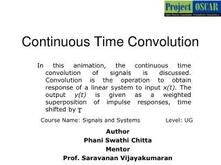
EE 313 Linear Systems and Signals Fall 2005. Continuous-Time Convolution. Prof. Brian L. Evans Dept. of Electrical and Computer Engineering The University of Texas at Austin. Initial conversion of content to PowerPoint by Dr. Wade C. Schwartzkopf. Useful Functions.

E N D
EE 313 Linear Systems and Signals Fall 2005 Continuous-Time Convolution Prof. Brian L. Evans Dept. of Electrical and Computer Engineering The University of Texas at Austin Initial conversion of content to PowerPointby Dr. Wade C. Schwartzkopf
Useful Functions • Unit gate function (a.k.a. unit pulse function) • What does rect(x / a) look like? • Unit triangle function rect(x) 1 x -1/2 0 1/2 D(x) 1 x -1/2 0 1/2
Unit Area -e e t Unit Impulse (Functional) • Mathematical idealism foran instantaneous event • Dirac delta as generalizedfunction (a.k.a. functional) Unit area: Sifting provided g(t) is defined at t = 0 Scaling: • Note that d(0) is undefined Unit Area -e e t
(1) Unit Area t 0 Unit Impulse (Functional) • Generalized sifting Assuming that a > 0 • By convention, plot Dirac delta as arrow at origin Undefined amplitude at origin Denote area at origin as (area) Height of arrow is irrelevant Direction of arrow indicates sign of area • With d(t) = 0 for t 0, it is tempting to think f(t) d(t) = f(0) d(t) f(t) d(t-T) = f(T) d(t-T) Simplify unit impulse under integration only
We can simplify d(t) under integration What about? Answer: 0 What about? By substitution of variables, Other examples What about at origin? Unit Impulse (Functional) Before Impulse After Impulse
Unit Impulse (Functional) • Relationship between unit impulse and unit step • What happens at the origin for u(t)? u(0-) = 0 and u(0+) = 1, but u(0) can take any value Common values for u(0) are {0, ½, 1} u(0) = ½ is used in impulse invariance filter design: L. B. Jackson, “A correction to impulse invariance,” IEEE Signal Processing Letters, vol. 7, no. 10, Oct. 2000, pp. 273-275.
LTI Systems • Recall for LTI system with input fand outputy • Homogeneity: cf(t) cy(t) • Time-invariance: cf(t-T) cy(t-T) • Adding additivity: • If a signal ( F(t) ) can be expressed as a sum of shifted ( t - Ti ) and weighted ( ci) copies of a simpler signal ( f(t) ), we easily find a system’s output ( Y(t) ) to that signal if we only know system’s output ( y(t) ) to that simpler signal • A common choice for f(t)is the impulse
Impulse Response • Impulse response of a system is response of the system to an input that is a unit impulse (i.e., a Dirac delta functional in continuous time) • Linear constant coefficient differential equation • When initial conditions are zero, this differential equation is LTI and system has impulse response b0 is coefficient (could be 0) of b0 DN f(t) on right-hand side N is highest order of derivative in differential equation
Impulse Response • In following plug, where did bn come from? • In solving these differential equations for t 0, • Funny things happen to y’(t) and y”(t) • In differential equations class, solved for m(t) • Likely ignored d(t) and d’(t) terms • Solution for m(t) is really valid for t 0+
F(t) t t=nDt Dt System Response • Signals as sum of impulses • But we know how to calculate the impulse response ( h(t) ) of a system expressed as a differential equation • Therefore, we know how to calculate the system output for any input, F(t)
Convolution Integral • Commonly used in engineering, science, math • Convolution properties • Commutative: f1(t) * f2(t) = f2(t) * f1(t) • Distributive: f1(t) * [f2(t) + f3(t)] = f1(t) * f2(t) + f1(t) * f3(t) • Associative: f1(t) * [f2(t) * f3(t)] = [f1(t) * f2(t)] * f3(t) • Shift: If f1(t) * f2(t) = c(t), thenf1(t) * f2(t - T) = f1(t - T) * f2(t) = c(t - T). • Convolution with impulse, f(t) * d(t) = f(t) • Convolution with shifted impulse, f(t) * d(t-T) = f(t-T) important later in modulation
Graphical Convolution Methods • From the convolution integral, convolution is equivalent to • Rotating one of the functions about the y axis • Shifting it by t • Multiplying this flipped, shifted function with the other function • Calculating the area under this product • Assigning this value to f1(t) * f2(t) at t
f(t) g(t) 3 2 * t t 2 -2 2 3 g(t-t) 2 f(t) t 2 -2 + t 2 + t Graphical Convolution Example • Convolve the following two functions: • Replace t with t in f(t) and g(t) • Choose to flip and slide g(t) since it is simpler and symmetric • Functions overlap like this:
3 g(t-t) 2 f(t) t 2 -2 + t 2 + t 3 g(t-t) 2 f(t) t 2 -2 + t 2 + t Graphical Convolution Example • Convolution can be divided into 5 parts • t < -2 • Two functions do not overlap • Area under the product of thefunctions is zero • -2 t < 0 • Part of g(t) overlaps part of f(t) • Area under the product of thefunctions is
3 g(t-t) 2 f(t) t 2 -2 + t 2 + t 3 g(t-t) 2 f(t) t 2 -2 + t 2 + t Graphical Convolution Example • 0 t < 2 • Here, g(t) completely overlaps f(t) • Area under the product is just • 2 t < 4 • Part of g(t) and f(t) overlap • Calculated similarly to -2 t < 0 • t 4 • g(t) and f(t) do not overlap • Area under their product is zero
Graphical Convolution Example • Result of convolution (5 intervals of interest): No Overlap Partial Overlap Complete Overlap Partial Overlap No Overlap y(t) 6 t -2 0 2 4