Download
1 / 54
560 likes | 761 Vues
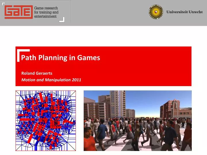
Path Planning in Games. Roland Geraerts Motion and Manipulation 2011. Path planning. Goal: bring characters from A to B Also vehicles, animals, camera, a formation,… Requirement: fast and flexible Real-time planning for thousands of characters Individuals and groups

E N D
Path Planning in Games Roland Geraerts Motion and Manipulation 2011
Path planning • Goal: bring characters from A to B • Also vehicles, animals, camera, a formation,… • Requirement: fast and flexible • Real-time planning for thousands of characters • Individuals and groups • Dealing with local hazards • Different types of environments • Requirement: visually convincing paths • The way humans move • Low energy usage (smooth, short, minimal rotation/acceleration) • Keep some distance (clearance) to obstacles • Social behavior (collision avoidance) • …
Do we need a new path planning algorithm? typical differences Nr. entities a few robots many characters Nr. DOFs many DOFs a few DOFs CPU time much time available little time available Interaction anti-social social Type pathnice path visually convincing path Algorithmscan be simple must be simple Correctness fool-proof may be incorrect
Path planning algorithms in games • Methods • Scripting • Networks of waypoints • Grid-based A* Algorithms • Navigation meshes • Local approaches • Flocking • Cheating
Methods: A* • Method • Construction phase: create a grid, mark free/blocked cells • Query phase: use A* to find the shortest path (in the grid) • Advantage • Simple • Disadvantages • Too slow in large scenes • Ugly paths • Little clearance to obstacles • Unnatural motions (sharp turns) • Fixed paths • Predictable motions
Methods: Potential Fields • Method • Goal generates attractive force • Obstacles generate repulsive force • Follow the direction of steepest descent of the potential toward the goal • Advantages • Flexibility to avoid local hazards • Smooth paths • Disadvantages • Expensive for multiple goals • Local minima
Methods: Probabilistic Roadmap Method • Method • Construction phase: build the roadmap • Query phase: query the roadmap • Advantages • Reasonably fast • High-dimensional problems • Disadvantages • Ugly paths • Fixed paths • Predictable motions • Lacks flexibility when environment changes
Methods: Probabilistic Roadmap Method • Method • Construction phase: build the roadmap • Query phase: query the roadmap • Advantages • Reasonably fast • High-dimensional problems • Disadvantages • Ugly paths • Fixed paths • Predictable motions • Lacks flexibility when environment changes
Methods: Navigation meshes • Method • Create a representation of the "walkable areas" of an environment • Extract the path • Advantages • General approach • Construction is fast due to use of GPU • Examples and source code can be found on http://code.google.com/p/recastnavigation • Disadvantages • Often needs a lot of manual editing • Current techniques are imprecise • Bad support for terrains Obstacles Walkable voxels Voxel regions Polygonal regions Convex regions A path
Methods: Navigation meshes • The state-of-the-art • Some open problems • Automatic annotation of the map • Areas: walk, climb, jump, crouch, “avoid” … • Special places: hiding and sniper spots, … • Handle large (dynamic) changes • Efficiently updating the data structure and paths • Improve the efficiency of mesh generation (large scenes) • Wrong coverage/connectivity due to confusing elements • Steep stairs, ramps, hills, curved surfaces, gaps • The mesh is only a data structure storing the walkable areas • How to create visually convincing paths?
Errors in path planning • Networks of waypoints are incorrect • Hand designed • Do not adapt to changes in the environment • Do not adapt to the type of character • Local methods fail to find a route • Keep stuck behind objects • Lead to repeated motion • Groups split up • Not planned as a coherent entity • Paths are unnatural • Not smooth • Stay too close to network/obstacles • Methodology is not general enough to handle all problems Titan Quest: Immortal throne
We need a fast generic framework • Representation of the free space • Planning algorithms
Representation of the free space • Comparison of navigation meshes
Generic representation free space • Input • Obstacles (points, lines and polygons) • Output: Explicit Corridor Map • Navigation mesh • Data structure: Medial axis + closest points Explicit Corridor Map (2D) Explicit Corridor Map (multi-layered)
Capturing the free space • Requirements of the data structure representing the free (walkable) space • Existence of a path • Contains all cycles • Short global paths, alternative paths • Provides high-clearance paths (corridors) • Provides maximum local flexibility • Small size • Fast extraction of paths • A good candidate • Generalized Voronoi Diagram + annotation
Voronoi Diagram • Some examples from nature maple leaf drying mud bacteria colonies wasps nest giraffe
Voronoi Diagram • Definitions • Voronoi region: set of all points closest to a given point • Voronoi diagram: union of all Voronoi regions Voronoi sites: (red) points
Voronoi Diagram • Approximation of the Voronoi Diagram • Compute a distance mesh for each point • Render each mesh in a different color by using the GPU • Using the Z-buffer, only pixels with the lowest distance values attribute to a pixel in the Frame buffer • A parallel projection of the meshes gives the diagram Perspective view (Z-buffer) Top view (Frame buffer)
Generalized Voronoi Diagram • Generalized Voronoi Diagram supports any type of obstacles • Point, disk, line, polygon, … • Convert concave polygons into convex ones, otherwise edges do not run into all corners
Generalized Voronoi Diagram • Generalized Voronoi Diagram supports any type of obstacles • Point, disk, line, polygon, … • Convert concave polygons into convex ones, otherwise edges do not run into all corners • Distance meshes • Point: cone • Disk: lifted cone • Line: tent + 2 cones • Polygon: n (point + line meshes) • Literature • [Hoff et al., 1999] • [Geraerts and Overmars, 2010]
From GDV to Medial axis • Generalized Voronoi Diagram (GVD) • Render distance meshes for each obstacle • Boundaries: bisectors between any two closest obstacles • Medial axis • Yields bisectors between any two distinct closest obstacles • Extraction of the medial axis • Edge: trace pixels between Voronoi regions; Convert them into bisector curves • Vertex: end point of an edge Medial axis GVD
Medial axis • The good • Existence of a path: full coverage/connectivity • Contains all cycles: yes • Provides high-clearance paths: yes • Small size: yes (linear) • Fast extraction of paths: yes • The bad • Unclear how to extract short(est) paths • Moving along 1D-curves limits flexibility • The ugly • Deal with robustness
Explicit Corridor Map • Basis: Medial Axis • Plus: annotated event points on the edges • Points where the object’s normals cross the bisector edge • Annotation: its two closest points on the obstacles • Bisector types • Straight lines versus parabola’s • Equals: planar subdivision (or navigation mesh) • Memory footprint The storage is linear in the number of obstacle vertices. • NoteThere is no need for storing pixels.
Explicit Corridor Map: experiments • Performance • Setup • NVIDIA GeForce 8800 GTX graphics card • Intel Core2 Quad CPU 2.4 GHz, 1 CPU used • Experiments • McKenna: 200x200 meter, 1600x1600 pixels, 23 convex polygons
Explicit Corridor Map: experiments • Performance • Setup • NVIDIA GeForce 8800 GTX graphics card • Intel Core2 Quad CPU 2.4 GHz, 1 CPU used • Experiments • McKenna: 200x200 meter, 1600x1600 pixels, 23 convex polygons time: 0.03s
Explicit Corridor Map: experiments • Performance • Setup • NVIDIA GeForce 8800 GTX graphics card • Intel Core2 Quad CPU 2.4 GHz, 1 CPU used • Experiments • City: 500x500 meter, 4000x4000 pixels, 548 convex polygons
Explicit Corridor Map: experiments • Performance • Setup • NVIDIA GeForce 8800 GTX graphics card • Intel Core2 Quad CPU 2.4 GHz, 1 CPU used • Experiments • City: 500x500 meter, 4000x4000 pixels, 548 convex polygons time: 0.3s
Explicit Corridor Map: experiments • Supports large environments • E.g. 1 km2 • Millimeter precision • However, there must be at leasttwo pixels in between two obstacles to discover an edge
Explicit Corridor Map: recent work • Extension to 2.5D (multi-layered) environments • Technique • Result (46 ms) Updated medial axes for Li and Lj Connection scene Multi-layered environment Partial medial axes for Li and Lj
Explicit Corridor Map: recent work • Handling dynamic changes • Technique for adding a point/line • Result (1 – 2.7 ms per update) A Finding closest site Continue in 1 dir. w1 has been reached Updated VD (point) Updated VD (line)
Explicit Corridor Map: recent work • Density-based crowd simulation
Explicit Corridor Map: some thoughts • Open questions • Dimensionality • How should we add height information? • How can we handle these extensions? • Terrains (elevation) • Different topological spaces • Different terrain types (grass, road, pavement) • How should we handle holes and enable jumping? Topological spaces: plane, sphere, cylinder, torus, Möbius strip, Klein bottle
Exploiting corridors • Extraction of a corridor (allows global path planning) • Retract the start and goal to the medial axis • Query the kd-tree • Connect the start and goal to the Corridor Map • Compute the shortest backbone path (using A*) Explicit Corridor Map Query Corridor with its backbone path
Exploiting corridors • The Corridor’s boundaries are given explicitly • Construction • Convenient representation • Small storage: linear in the number of eventspoints • Computation of closest points in O(1) time (on average) • Allows computing shortest minimum-clearance paths
Explicit Corridors: Obtaining clearance • Minimum clearance in explicit corridors • For each closest point cp, move cp toward its center point c • The displacement equals the desired clearance clmin • Insert event point(s) if clmin > distance(c, cp) c cp Explicit Corridor Shrunk corridors Shrinking a corridor
Explicit Corridors: Shortest paths • Computing the shortest path • Construct a triangulation • 2ith triangle: (li , ri , li+1) ; 2i+1th triangle: (ri , li+1 , ri+1) • If the start [goal] is not included, add triangle (s, l1 , r1) [(ln , rn ,g)] • Compute the shortest path • Funnel algorithm [Guibas et al. 1987] ri+1 li+1 g ri li s Triangulation Shortest path Explicit Corridor
Explicit Corridors: Shortest paths • Sketch of the Funnel algorithm • Funnel • Tail: computed shortest path from start to apex • Fan: 2 outward convex chains plus one diagonal • The fan keeps track of all possible shortest paths • Algorithm • Add diagonals iteratively whileupdating the funnel • Algorithm is linear in the number of diagonals • (or events) start tail apex fan diagonal goal
Explicit Corridors: Shortest paths • Computing the shortest minimum clearance path • Shrink the corridor • Construction time: linear in the number of event points • Compute the shortest path • Adjust Funnel algorithm to deal with circular arcs • Construction time: linear in the number of event points Left/right closest points Triangulation Shortest path
The Indicative Route Method • A path planning algorithm should NOT compute a path • A one-dimensional path limits the character’s freedom • Humans don’t do that either • It should produce • An Indicative/Preferred Route • Guides character to goal • A corridor • Provides a global route • Allows for flexibility
The Indicative Route Method • ‘Algorithm’ • Compute a collision free indicative route from A to B • Compute a corridor containing the route • Move an attraction point along the indicative route • The attraction point attracts the character • The corridor’s boundary push thecharacter away • Other characters push the character away
The Indicative Route Method • Boundary force • Find closest point on corridor boundary • Perpendicular to boundary • Increases to infinity when closer to boundary • Force is 0 when clearance is large enough • Steering force • Towards attraction point • Can be constant • Obtain path • Force leads to an acceleration term • Integration over time, update velocity/position/attraction point • Yields a smooth (C1-continuous) path
The Indicative Route Method • Resulting vector field • Indicative Route is smooth path
The Indicative Route Method • Examples • Adding/changing forces leads to other “behavior” Smooth path Short path Obstacle avoidance Obstacle avoidance (Helbing model) + path variation = crowd? • Distinguish three scales1. Macro (corridor)2.Meso (indicative route)3. Micro (local behavior) Coherent groups Path variation Camera path
The Indicative Route Method • Examples • Adding/changing forces leads to other “behavior” Stealth-based path planning
The Indicative Route Method • Experiments • Setup • Intel Core2 Quad CPU 2.4 GHz, 1 CPU • Experiments • City: 500x500 meter, 1.000 random queries • Results (average query time)
The Indicative Route Method • Experiments • Setup • Intel Core2 Quad CPU 2.4 GHz, 1 CPU • Experiments • City: 500x500 meter, 1 query • Results (query time) • 2.8 ms ECM (0.3s) Explicit corridor Shrunk corridor Triangulation Shortest path Smooth path
Conclusion • Advantages • Fast and flexible planner creates visually convincing paths • Computation of smooth, short minimum clearance paths • The algorithms run in linear time and are fast • The algorithms are simple • Open problems • Automatic annotation of the navigation mesh • Handling 3D spaces • Handling character behavior • E.g. shopping and beach behavior • Interaction between different entities (human, car, bicycle)
Collision-avoidance model • Particle-based approaches • E.g. Helbing model • When characters get close to each other they push each other away • Force depends on the distance between their personal spaces and whether they can see each other • Disadvantages • Reaction is late • Also reaction when no collision • Artifacts Goal force Avoidance force Resulting force
Improved collision-avoidance model • Collision-predication approach • When characters are on collision course we compute the positions at impact (of personal spaces) • Direction depends on their relative position at impact • Force depends on the distance to impact • Care must be taken when combining forces Goal force Avoidance force Resulting force