Download

1 / 70
700 likes | 710 Vues
Computing Environment. The computing environment rapidly evolving ‑ you need to know not only the numerical methods, but also How and when to apply them, Which computers to use, What type of code to write, What kind of CPU time and memory your jobs will need,

E N D
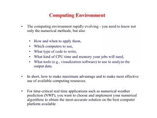
Computing Environment • The computing environment rapidly evolving ‑ you need to know not only the numerical methods, but also • How and when to apply them, • Which computers to use, • What type of code to write, • What kind of CPU time and memory your jobs will need, • What tools (e.g., visualization software) to use to analyze the output data. • In short, how to make maximum advantage and to make most effective use of available computing resources. • For time-critical real time applications such as numerical weather prediction (NWP), you want to choose and implement your numerical algorithms to obtain the most-accurate solution on the best computer platform available
Definitions – Clock Cycles, Clock Speed • The clock rate is the fundamental rate in cycles per second (measured in hertz) at which a computer performs its most basic operations. Often measured in nanoseconds (ns) or megahertz. The clock rate of a CPU is normally determined by the frequency of an oscillator crystal. • The first commercial PC, the Altair (by MITS), used an Intel 8080 CPU with a clock rate of 2 MHz. • The original IBM PC (1981) had a clock rate of 4.77 MHz. • In 1995, Intel's Pentium chip ran at 100 MHz (100 million cycles/second). • In 2002, an Intel Pentium 4 model was introduced as the first CPU with a clock rate of 3 GHz. • 3600 MegaHz (MHz) = 3.6 GigaHz (GHz) (fastest Pentium IV) ~ clock speed of 0.3 nanosecond (ns) • 1600 mhz Itanium 2 ~ 0.6 ns clock speed • Heard of over-clocking? Run the CPU at a higher rate than vendor specification.
Significance of Clock Speed • Clock speed is not everything. • May take several clocks to do one multiplication • May perform many operations per clock • Memory access also takes time, not just computation • mHz is not the only measure of CPU speed. Different CPUs of the same mHz often differ in speed. E.g., the 1.6GHz Itanium 2, Intel’s 64bit processor, is faster than the 3.6GHz Pentium 4. So are the latest generation Intel Core 2 architecture CPUs (has lower clock rate than P4). AMD’s (e.g., Athlon 64 X2) and Intel’s processors (e.g., Core 2 Dual) can no be directly compared based on clock speed. • The clock rate of the computer's front side bus, the clock rate of the RAM, the width in bits of the CPU's memory bus, and the amount of Level 1, Level 2 and Level 3 cache also affect a computer’s speed. Other factors include video card, disk drive speeds. • The current generation Intel processors, e.g., Core 2, has lower MHz than Pentium IV but higher processing power – larger Level-2 cache is one reason.
Significance of Clock Speed – additional comments • Comparing • The clock rate of a computer is only useful for providing comparisons between computer chips in the same processor family. An IBM PC with an Intel 486 CPU running at 50 MHz will be about twice as fast as one with the same CPU, memory and display running at 25 MHz, while the same will not be true for MIPS R4000 running at the same clock rate as the two are different processors with different functionality. Furthermore, there are many other factors to consider when comparing the speeds of entire computers, like the clock rate of the computer's front side bus, the clock rate of the RAM, the width in bits of the CPU's bus and the amount of Level 1, Level 2 and Level 3 cache. • Clock rates should not be used when comparing different computers or different processor families. Rather, some software benchmark should be used. Clock rates can be very misleading since the amount of work different computer chips can do in one cycle varies. For example, RISC CPUs tend to have simpler instructions than CISC CPUs (but higher clock rates), and superscalar processors can execute more than one instruction per cycle, yet it is not uncommon for them to do "less" in a clock cycle. • History • In the early 1990s, most computer companies advertised their computers' speed chiefly by referring to their CPUs' clock rates. This led to various marketing games, such as Apple Computer's decision to create and market the Power Macintosh 8100/110 with a clock rate of 110 MHz so that Apple could advertise that its computer had the fastest clock speed available -- the fastest Intel processor available at the time ran at 100 MHz. This superiority in clock speed, however, was meaningless since the PowerPC and Pentium CPU architectures were completely different. The Power Mac was faster at some tasks but slower at others. • After 2000, Intel's competitor, AMD, started using model numbers instead of clock rates to market its CPUs because of the lower CPU clocks when compared to Intel. Continuing this trend it attempted to dispell the "Megahertz myth" which it claimed did not tell the whole story of the power of its CPUs. In 2004, Intel announced it would do the same, probably because of consumer confusion over its Pentium M mobile CPU, which reportedly ran at about half the clock rate of the roughly equivalent Pentium 4 CPU. As of 2007, performance improvements have continued to come through innovations in pipelining, instruction sets, and the development of multi-core processors, rather than clock speed increases (which have been constrained by CPU power dissipation issues). However, the transistor count has continued to increase as predicted by Moore's Law.
Definitions – FLOPS • Floating Operations / Second • Megaflops – million (106) FLOPS • Gigaflops – billion (109) FLOPS • Teraflops – trillion (1012) FLOPS • Petaflops – quadrillion (1015) FLOPS • The fastest computer system since 2005 can achieve over 100 TFlops sustained – see http://www.top500.org). • A good measure of code performance – typically one add is one flop, one multiplication is also one flop • Cray J90 Vector processor (that OU used to own) theoretical peak speed = 200 Mflops, most codes achieves only 1/3 of peak • Fastest US-made vector supercomputer CPU - Cray T90 peak = 3.2 Gflops • NEC XS-5 Vector CPU Used in Earth Simulator of Japan (the fastest computer in the world in 2003) = 8 Gflops • Fastest non-vector or super-scalar processors (e.g., Intel Itanium 2 processors), have peak speed of over 10 Gflops. • The 3.2 GHz Pentium IV Xeon processor in OSCER Topdawg has theoretical peak speed of 6.5Gflops. • See http://www.specbench.org for the latest benchmarks of processors for real world problems. Specbench numbers are relative.
MIPS • Million instructions per second – also a measure of computer speed – used most in the old days when computer architectures were relatively simple • MIPS is hardly used these days because the number of instructions used to complete one FLOP is very much CPU dependent with today’s CPUS
Register • A, special, high-speed storage area within the CPU. All data must be represented in a register before it can be processed. For example, if two numbers are to be multiplied, both numbers must be in registers, and the result is also placed in a register. • The number of registers that a CPU has and the size of each (number of bits) help determine the power and speed of a CPU. For example a 32-bit CPU is one in which each register is 32bits wide. Therefore, each CPU instruction can manipulate 32 bits of data. • Usually, the movement of data in and out of registers is completely transparent to users, and even to programmers. Only assembly language programs can manipulate registers. In high-level languages, the compiler is responsible for translating high-level operations into low-level operations that access registers.
Cache • Pronounced cash, a special high-speed storage mechanism. It can be either a reserved section of main memory or an independent high-speed storage device. • Two types of caching are commonly used in PCs:memory caching and disk caching. A memory cache, sometimes called a cache store or RAM cache, is a portion of memory made of high-speed static RAM (SRAM) instead of the slower and cheaper dynamic RAM (DRAM) used for main memory. • Memory caching is effective because most programs access the same data or instructions over and over. By keeping as much of this information as possible in SRAM, the computer avoids accessing the slower DRAM. • Some memory caches are built into the architecture of microprocessors. The Intel 80486 microprocessor, for example, contains an 8K memory cache, and the Pentium has a 16K cache. Today’s Intel Core-2 processors have 2-4 mb caches. Such internal caches are often called Level 1 (L1) caches. Most modern PCs also come with external cachememory (often also located on the CPU die), called Level 2 (L2) caches. These caches sit between the CPU and the DRAM. Like L1 caches, L2 caches are composed of SRAM but they are much larger. Some CPUs even have Level 3 caches. (Note most latest generation CPUs build L2 caches on CPU dies, running at the same clock rate as CPU). • Disk caching works under the same principle as memory caching, but instead of using high-speed SRAM, a disk cache uses conventional main memory. The most recently accessed data from the disk (as well as adjacent sectors) is stored in a memory buffer. When a program needs to accessdata from the disk, it first checks the diskcache to see if the data is there. Disk caching can dramatically improve the performance of applications, because accessing a byte of data in RAM can be thousands of times faster than accessing a byte on a hard disk. Today’s hard drives often have 8 – 16 mb memory caches. • When data is found in the cache, it is called a cache hit, (versus cache miss) and the effectiveness of a cache is judged by its hit rate. Many cache systems use a technique known as smart caching, in which the system can recognize certain types of frequently used data. The strategies for determining which information should be kept in the cache constitute some of the more interesting problems in computer science.
Storage and Memory • They refer to storage areas in the computer. The term memory identifies data storage that comes in the form of chips, and the word storage is used for memory that exists on tapes or disks. • Moreover, the term memory is usually used as a shorthand for physicalmemory, which refers to the actual chips capable of holding data. Some computers also use virtual memory, which expands physical memory onto a hard disk. • Every computer comes with a certain amount of physical memory, usually referred to as main memory or RAM. • Today’s computers also come with hard disk drives that are used to store permanent data. • The content in memory is usually lost when the computer is powered down, unless it’s flash memory (as in your thumb drives or iPod) but data on hard drives are not. • The earliest PCs did not have hard drives – they store data on and boot from floppy disks.
What’s an Instruction? • Load a value from a specific address in main memory into a specific register • Store a value from a specific register into a specific address in main memory • Add two specific registers together and put their sum in a specific register – or subtract, multiply, divide, square root, etc • Determine whether two registers both contain nonzero values (“AND”) • Jump from one sequence of instructions to another (branch) • … and so on
Memory or Data Unit • A bit is a binary digit, taking a value of either 0 or 1 . • For example, the binary number 10010111 is 8 bits long, or in most cases, one modern PC byte. Typically, 1 byte = 8 bits • Binary digits are a basic unit of information storage and communication in digital computing and digital information theory. • Fortran single precision floating point numbers on most computers consist of 32 bits, or 4 bytes. • Quantities of bits • kilobit (kb) 103 • megabit (Mb) 106 • gigabit (Gb) 109 • terabit (Tb) 1012 • petabit (Pb) 1015 • exabit (Eb) 1018 • zettabit (Zb) 1021 • yottabit (Yb) 1024
Bandwidth • The speed at which data flow across a network or wire • 56K Modem = 56 kilobits / second • T1 link = 1.554 mbits / sec • T3 link = 45 mbits / sec • FDDI = 100 mbits / sec • Fiber Channel = 800 mbits /sec • 100 BaseT (fast) Ethernet = 100 mbits/ sec • Gigabit Ethernet = 1000 mbits /sec max • Wireless 802.11g = 54 mbits/sec max • Wireless 802.11n = 248 mbits/sec max • USB 1.1 = 12 mbits/sec, USB 2.0 = 480 mbits/sec • Brain system = 3 Gbits / s • 1 byte = 8 bits • When you see kb/second, find out if b means bit or byte!
Central Processing Unit • Also called CPU or processor: the “brain” • Parts • Control Unit: figures out what to do next -- e.g., whether to load data from memory, or to add two values together, or to store data into memory, or to decide which of two possible actions to perform (branching) • Arithmetic/Logic Unit: performs calculations – e.g., adding, multiplying, checking whether two values are equal • Registers: where data reside that are directly processed and stored by the CPU • Modern CPUs usually also contain on-die Level-1, Level-2 caches and sometimes Level-3 cache too, very fast forms of memory.
Hardware Evolution • Mainframe computers • Vector Supercomputers • Workstations • Microcomputers / Personal Computers • Desktop Supercomputers • Workstation Super Clusters • Supercomputer Clusters • Portables • Handheld, Palmtop, cell phones, et al….
Types of Processors • Scalar (Serial) • One operation per clock cycle • Vector • Multiple operations per clock cycle. Typically achieved at the loop level where the instructions are the same or similar for each loop index • Superscalar (most of today’s microprocessors) • Several operations per clock cycle
Types of Computer Systems • Single Processor Scalar (e.g., ENIAC, IBM704, traditional IBM-PC and Mac) • Single Processor Vector (CDC7600, Cray-1) • Multi-Processor Vector (e.g., Cray XMP, C90, J90, T90, NEC SX-5, SX-6), • Single Processor Super-scalar (most desktop PCs today) • Multi-processor scalar (early multi-processor workstations) • Multi-processor super-scalar (e.g., SOM Sun Enterprise Server Rossby, IBM Regata of OSCER Sooner, Xeon workstations and dual-core PCs) • Clusters of the above (e.g., OSCER Linux cluster Topdawg – cluster of 2-CPU Pentium IV Linux Workstations essentially, Earth Simulator – Cluster of multiple vector processor nodes)
ENIAC – World’s first electronic computer (1946-1955) • The world's first electronic digital computer, Electronic Numerical Integrator and Computer (ENIAC), was developed by Army Ordnance to compute World War II ballistic firing tables. • ENIAC’s thirty separate units, plus power supply and forced-air cooling, weighed over thirty tons. It had 19,000 vacuum tubes, 1,500 relays, and hundreds of thousands of resistors, capacitors, and inductors and consumed almost 200 kilowatts of electrical power. • See story at http://ftp.arl.mil/~mike/comphist/eniac-story.html
ENIAC – World’s first electronic computer (1946-1955) Fromhttp://ftp.arl.army.mil/ftp/historic-computers
ENIAC – World’s first electronic computer (1946-1955) From http://ftp.arl.army.mil/ftp/historic-computers
Cray-1, the first ‘vector supercomputer’, 1976 • Single vector processor • 133 MFLOPS peak speed • 1 million 8 byte words = 8mb of memory • Price $5-8 million • Liquid cooling system using Freon • Right, Cray 1A on exhibit at NCAR
Cray-J90 • Air-cooled, low-cost vector supercomputers introduced by Cray in the mid-'90s. • OU owned a 16-processor J90. Decommissioned until early 2003.
Cray-T90, the last major shared-memory parallel vector supercomputer made by US Company • Up to 32 vector processors • 1.76 GFLOPS/CPU • 512MW = 4 GB memory • Decommissioned from San Diego Supercomputer Center in March 2002 • See Historic Cray Systems at http://www.cray-cyber.org/general/start.php
Memory Architectures • Shared Memory Parallel (SMP) Systems • Distributed Memory Parallel (DMP) Systems • Memory can be accessed and addressed • uniformly by all processors with no user intervention • Usually use fast/expensive CPU, Memory, and networks • Easier to use • Difficult to scale to many (> 32) processors • Emerging multi-core processors will surely share memory, and in some cases even cache. • Each processor has its own memory • Others can access its memory only via • network communications • Often off-the-shelf components, • therefore low cost • Harder to use, explicit user specification of • communications often needed. • Not suitable for inherently serial codes • High-scalability - largest current system • has many thousands of processors – massively parallel systems
Memory Architectures • Multi-level memory (cache and main memory) architectures • Cache – fast and expensive memory • Typical L1 cache size in current day microprocessors ~ 32 K • L2 size ~ 256K to 16mb (P4 has 512K to 2 mb) • Main memory a few Mb to many Gb. • Try to reuse the content of cache as much as possible before the content is replaced by new data or instructions • Disk, CD ROM etc – the slowest forms of memory – still direct access • Tapes, even slower, serial access only many newer processors have L2 Cache on CPU die also Disk etc
OSCER Hardware: IBM Regatta (Decommissioned) 32 Power4 CPUs 32 GB RAM 200 GB disk OS: AIX 5.1 Peak speed: 140 billion calculations per second Programming model: shared memory multithreading
OSCER IBM Regatta p690 Specs – sooner.ou.edu • 32 Power4 processors running at 1.1 GHz • 32 GB shared memory. Distributed memory parallelization is also supported via message passing (MPI) • 3 levels of cache. 32KB L1 cache per CPU, 1.41MB L2 cache shared by each two CPUs on the same die (dual-core processors), and 128mb L3 cache shared by eight processors. • The peak performance of each processor is 4.4 GFLOPS (4 FLOPS per cycle).
IBM p-Series server (sooner) architecture – Power4 CPU chip(from http://www.redbooks.ibm.com/pubs/pdfs/redbooks/sg247041.pdf)
IBM p-Series server (sooner) architecture(from http://www.redbooks.ibm.com/pubs/pdfs/redbooks/sg247041.pdf)
OSCER Linux Cluster Specs – Topdawg.oscer.ou.edu • Intel Pentium-4 Xeon EM64T processors running at 3.2 GHz, peak 6.5 Gflops • Each node contains 2 CPUs, each node has 4GB memory • Each processor has 2mb L-2 cache • Interconnet: InfiniBand (primary, 5 Gbps, latency 3 ms) and 1000Mbps Ethernet (backup, 976 Mbps, latency 9 ms) • 512 dual-processor computer nodes • Total theoretical peak performance 6.6 Teraflops • System: Redhat Linux Enterprise 4.0. • See also http://www.oscer.ou.edu/docs/hardsoft_dell_cluster_pentium4xeon.php for additional information
Parallelism • Parallelism means doing multiple things at the same time: you can get more work done in the same time.
Instruction Level Parallelization • Superscalar: perform multiple operations at a time • Pipeline: start performing an operation on one piece of data while finishing the same operation on another piece of data • Superpipeline: perform multiple pipelined operations at the same time • Vector: load multiple pieces of data into special registers in the CPU and perform the same operation on all of them at the same time
What’s an Instruction? • Load a value from a specific address in main memory into a specific register • Store a value from a specific register into a specific address in main memory • Add two specific registers together and put their sum in a specific register – or subtract, multiply, divide, square root, etc • Determine whether two registers both contain nonzero values (“AND”) • Jump from one sequence of instructions to another (branch) • … and so on
Scalar Operation z = a * b + c * d • Loadainto registerR0 • LoadbintoR1 • MultiplyR2 = R0 * R1 • LoadcintoR3 • LoaddintoR4 • MultiplyR5 = R3 * R4 • AddR6 = R2 + R5 • StoreR6intoz How would this statement be executed? Takes 10 operationsto complete thecalculations
Does Order Matter? z = a * b + c * d • LoadaintoR0 • LoadbintoR1 • MultiplyR2 = R0 * R1 • LoadcintoR3 • LoaddintoR4 • MultiplyR5 = R3 * R4 • AddR6 = R2 + R5 • StoreR6intoz LoaddintoR4 LoadcintoR3 MultiplyR5 = R3 * R4 LoadaintoR0 LoadbintoR1 MultiplyR2 = R0 * R1 AddR6 = R2 + R5 StoreR6intoz In the cases where order doesn’t matter, we say that the operations are independent of one another.
Superscalar Operation z = a * b + c * d • LoadaintoR0 ANDloadbintoR1 • MultiplyR2 = R0 * R1 ANDloadcintoR3 AND loaddintoR4 • MultiplyR5 = R3 * R4 • AddR6 = R2 + R5 • StoreR6intoz So, we go from 8 operations down to 5.
Superscalar Loops DO i = 1, n z(i) = a(i)*b(i) + c(i)*d(i) END DO !! i = 1, n Each of the iterations is completely independent of all of the other iterations; e.g., z(1) = a(1)*b(1) + c(1)*d(1) has nothing to do with z(2) = a(2)*b(2) + c(2)*d(2) Operations that are independent of each other can be performed in parallel.
Superscalar Loops for (i = 0; i < n; i++) { z[i] = a[i]*b[i] + c[i]*d[i]; } /* for i */ • Loada[i]intoR0ANDloadb[i]intoR1 • Multiply R2 = R0 * R1 ANDload c[i] into R3 ANDload d[i] into R4 • Multiply R5 = R3 * R4 ANDload a[i+1] into R0 ANDload b[i+1] into R1 • Add R6 = R2 + R5 ANDloadc[i+1]intoR3ANDloadd[i+1]intoR4 • StoreR6intoz[i]ANDmultiplyR2 = R0 * R1 • etc etc etc
Example: IBM Power4 8-way superscalar: can execute up to 8 operations at the same time • 2 integer arithmetic or logical operations, and • 2 floating point arithmetic operations, and • 2 memory access (load or store) operations, and • 1 branch operation, and • 1 conditional operation
Pipelining Pipelining is like an assembly line. • An operation consists of multiple stages. • After a set of operands complete a particular stage, they move into the next stage. • Then, another set of operands can move into the stage that was just abandoned.
Instruction Fetch Instruction Fetch Instruction Fetch Instruction Fetch Instruction Decode Instruction Decode Instruction Decode Instruction Decode Operand Fetch Operand Fetch Operand Fetch Operand Fetch Instruction Execution Instruction Execution Instruction Execution Instruction Execution Result Writeback Result Writeback Result Writeback Result Writeback Pipelining Example t = 2 t = 5 t = 0 t = 1 t = 3 t = 4 t = 6 t = 7 i = 1 i = 2 i = 3 i = 4 Computation time If each stage takes, say, one CPU cycle, then once the loop gets going, each iteration of the loop only increases the total time by one cycle. So a loop of length 1000 takes only 1004 cycles, instead of 5000 for the above example.
Superpipelining Superpipelining is a combination of superscalar and pipelining. So, a superpipeline is a collection of multiple pipelines that can operate simultaneously. In other words, several different operations can execute simultaneously, and each of these operations can be broken into stages, each of which is filled all the time. For example, z = a * b + c * d can employ superscalar operations (reducing operations counts from 8 to 5), and pipelining can be achieved at the loop level (as in previous slide) So you can get multiple operations per CPU cycle. For example, a IBM Power4 can have over 200 different operations “in flight” at the same time.
Vector Processing • The most powerful CPUs or processors (e.g., NEC SX-6) are vector processors that can perform operations on a stream of data in a pipelined fashion – so vectorization is one type of pipelining. • A vector here is defined as an ordered list of scalar values. For example, an array stored in memory is a vector. • Vector systems have machine instructions (vector instructions) that fetch a vector of values (instead of single ones) from memory, operate on them and store them back to memory. • Basically, vector processing is a version of the Single Instruction Multiple Data (SIMD) parallel processing technique. • On the other hand, scalar processing usually requires one instruction to act on each data value.
Vector Processing • A vector processor, or array processor, is a CPU design that is able to run mathematical operations on multiple data elements simultaneously. This is in contrast to a scalar processor which handles one element at a time. • The vast majority of CPUs are scalar (or close to it). Vector processors were common in the scientific computing area, where they formed the basis of most supercomputers through the 1980s and into the 1990s, but general increases in performance and processor design saw the near disappearance of the vector processor as a general-purpose CPU. • Today commodity CPU designs include some vector processing instructions, typically known as SIMD (Single Instruction, Multiple Data), like SSE (Streaming SIMD Extensions) and AltiVec. • Modern Video game consoles and consumer computer-graphics hardware in particular rely heavily on vector processors in their architecture. In 2000, IBM, Toshiba and Sony collaborated to create a Cell processor, consisting of one scalar processor and eight vector processors, for the Sony PlayStation 3.
History of Vector Processing • Vector processing was first worked on in the early 1960s at Westinghouse in their Solomon project. Solomon's goal was to dramatically increase math performance by using a large number of simple math co-processors (or ALUs) under the control of a single master CPU. The CPU fed a single common instruction to all of the ALUs, one per "cycle", but with a different data point for each one to work on. This allowed the Solomon machine to apply a single algorithm to a large data set, fed in the form of an array. In 1962 Westinghouse cancelled the project, but the effort was re-started at the University of Illinois as the ILLIAC IV. Their version of the design originally called for a 1 GFLOPS machine with 256 ALUs, but when it was finally delivered in 1972 it had only 64 ALUs and could reach only 100MFLOPS. Nevertheless it showed that the basic concept was sound, and when used on data-intensive applications, such as computational fluid dynamics, the "failed" ILLIAC was the fastest machine in the world. • The first successful implementation of a vector processor appears to be the CDC STAR-100 and the Texas Instruments Advanced Scientific Computer. The basic ASC (i.e., "one pipe") ALU used a pipeline architecture which supported both scalar and vector computations, with peak performance reaching approximately 20 MOPS or MFLOPS, readily achieved when processing long vectors. Expanded ALU configurations supported "two pipes" or "four pipes" with a corresponding 2X or 4X performance gain. Memory bandwidth was sufficient to support these expanded modes. The STAR was otherwise slower than CDC's own supercomputers like the CDC 7600, but at data related tasks they could keep up while being much smaller and less expensive. However the machine also took considerable time decoding the vector instructions and getting ready to run the process, so it required very specific data sets to work on before it actually sped anything up. • The technique was first fully exploited in the famous Cray-1. Instead of leaving the data in memory like the STAR and ASC, the Cray design had eight "vector registers" which held sixty-four 64-bit words each. The vector instructions were applied between registers, which is much faster than talking to main memory. In addition the design had completely separate pipelines for different instructions, for example, addition/subtraction was implemented in different hardware than multiplication. This allowed a batch of vector instructions themselves to be pipelined, a technique they called vector chaining. The Cray-1 normally had a performance of about 80 MFLOPS, but with up to three chains running it could peak at 240 MFLOPS – a respectable number even today. • Other examples followed. CDC tried once again with its ETA-10 machine, but it sold poorly and they took that as an opportunity to leave the supercomputing field entirely. Various Japanese companies (Fujitsu, Hitachi and NEC) introduced register-based vector machines similar to the Cray-1, typically being slightly faster and much smaller. Oregon-based Floating Point Systems (FPS) built add-on array processors for minicomputers, later building their own minisupercomputers. However Cray continued to be the performance leader, continually beating the competition with a series of machines that led to the Cray-2, Cray X-MP and Cray Y-MP. Since then the supercomputer market has focused much more on massively parallel processing rather than better implementations of vector processors. However, recognizing the benefits of vector processing IBM developed Virtual Vector Architecture for use in supercomputers coupling several scalar processors to act as a vector processor. • Today the average computer at home crunches as much data watching a short QuickTime video as did all of the supercomputers in the 1970s. Vector processor elements have since been added to almost all modern CPU designs, although they are typically referred to as SIMD. In these implementations the vector processor runs beside the main scalar CPU, and is fed data from programs that know it is there.
Processor board of a CRAY YMP • Processor board of a CRAY YMP vector computer (operational ca. 1992-2000). The board was liquid cooled and is one vector processor with shared memory (access to one central memory)
Vector Processing - Example DO I = 1, N A(I) = B(I) + C(I) ENDDO • If the above code is vectorized, the following processes will take place, • A vector of values in B(I) will be fetched from memory. • A vector of values in C(I) will be fetched from memory. • A vector add instruction will operate on pairs of B(I) and C(I) values. • After a short start-up time, stream of A(I) values will be stored back to memory, one value every clock cycle. • If the code is not vectorized, the following scalar processes will take place, • B(1) will be fetched from memory. • C(1) will be fetched from memory. • A scalar add instruction will operate on B(1) and C(1). • A(1) will be stored back to memory • Step (1) to (4) will be repeated N times.
Vector Processing • Vector processing allows a vector of values to be fed continuously to the vector processor. • If the value of N is large enough to make the start-up time negligible in comparison, on the average the vector processor is capable of producing close to one result per clock cycle (imaging the automobile assembly line)
Vector Processing • If the same code is not vectorized (using J90 as an example), for every I iteration, e.g. I=1, a clock cycle each is needed to fetch B(1) and C(1), about 4 clock cycles are needed to complete a floating-point add operation, and another clock cycle is needed to store the value A(1). • Thus a minimum of 6 clock cyclesare needed to produce one result (complete one iterations). • We can say that there is a speed up of about 6 times for this example if the code is vectorized.
Vector Processing • Vector processors can often chain operations such as add and multiplication together (because they have multiple functional units, for add, multiply etc), in much the same way as superscalar processor does, so that both operations can be done in one clock cycles. This further increases the processing speed. • It usually helps to have long statements inside vector loops in this case.