Download
1 / 37
460 likes | 840 Vues
t -tests, ANOVA & Regression. Andrea Banino & Punit Shah . Background: t-tests. Samples vs Populations Descriptive vs Inferential William Sealy Gosset (‘Student’) Distributions, probabilities and P-values Assumptions of t-tests. P-values .

E N D
t-tests, ANOVA & Regression Andrea Banino & Punit Shah
Background: t-tests • Samples vs Populations • Descriptive vs Inferential • William Sealy Gosset (‘Student’) • Distributions, probabilities and P-values • Assumptions of t-tests
P-values • P values = the probability that the observed result was obtained by chance • i.e. when the null hypothesis is true • αlevel is set a priori (Usually .05) • If p < .05 level then we reject the null hypothesis and accept the experimental hypothesis • 95% certain that our experimental effect is genuine • If however, p > .05 level then we reject the experimental hypothesis and accept the null hypothesis
Research Example • Is there different activation of the FFG for faces vs objects • Within-subjects design: Condition 1: Presented with face stimuli Condition 2: Presented with object stimuli Hypotheses • H0 = There is no difference in activation of the FFG during face vs object stimuli • HA =There is a significant difference in activation of the FFG during face vs object stimuli
Results- How to compare? • Mean BOLD signal change during object stimuli = +0.001% • Mean BOLD signal change during facial stimuli = +4% • Great- there is a difference, but how do we know this was not just a fluke?
Compare the mean between 2 conditions (Faces vs Objects) • H0: μA = μB (null hypothesis)- no difference in brain activation between these 2 groups/conditions • HA: μA ≠ μB (alternative hypothesis) = there is a difference in brain activation between these 2 groups/conditions • if 2 samples are taken from the same population, then they should have fairly similar means if 2 means are statistically different, then the samples are likely to be drawn from 2 different populations, i.ethey really are different BOLD response Condition 1 (Objects) Condition 2 (Faces)
Condition 1(Objects) Condition 2 (Faces) Calculating t * Independent Samples t-test • t = differences between sample means / standard error of sample means • The exact equation varies depending on which type of t-test used BOLD response
Types of t-test & Alternatives • 1 Sample t-test (sample vs. hypothesized mean) • 2 Sample t-test (group/condition 1 vs group/condition 2)
Degrees of Freedom ( df) • The number of ‘entities’ that are free to vary when estimating t • n – 1 (for paired sample t) • Larger sample or no. of observations = more df Putting it all together… • t (df) = t= t-value, p = p-value
Application to fMRI? Subtraction / Multiple subtraction Techniques • compare the means and standard deviations between various conditions • each voxel considered an ‘n’ – so Bonferroni correction is made for the number of voxels compared Time
How are t-tests/ANOVA relevant to fMRI? Image time-series Statistical Parametric Map Design matrix Spatial filter Realignment Smoothing General Linear Model StatisticalInference RFT Normalisation p <0.05 Anatomicalreference Parameter estimates
t-tests in Statistical Parametric Mapping • GLM: Y= X β + ε • 2nd level analysis • β1 is an estimate of signal change over time attributable to the condition of interest (face vs object) • Set up contrast (cT) 1 0 for β1:1xβ1+0xβ2+0xβn/s.d • Null hypothesis: cTβ=0 No significant effect at each voxel for condition β1 • Contrast 1 -1 : Is the difference between 2 conditions significantly non-zero? • t = cTβ/sd[cTβ] • t-tests are simple combinations of the betas; they are either positive or negative (b1 – b2 is different from b2 – b1)
c’ = 1 0 0 0 0 0 0 0 SPM{t} T test - one dimensional contrasts – SPM {t } A contrast = a weighted sum of parameters: c´ ´ b b1 > 0 ? Compute 1xb1+ 0xb2+ 0xb3+ 0xb4+ 0xb5+ . . .= c’b c’ = [1 0 0 0 0 ….] b1b2b3b4b5.... divide by estimated standard deviation of b1 contrast ofestimatedparameters c’b T = T = varianceestimate s2c’(X’X)-c
ANOVA- Analysis of Variance • More that 2 groups and/or conditions- e.g. objects, faces and bodies • Do this without inflating the Type I error rate • Still compares the differences in means between groups/conditions but it uses the variance of data to calculate if means are significantly different (HA) • Tests the null hypothesis that the means are the same via the F- test • Extra assumptions
How? The F- statistic F-ratio = MSM / MSR • By comparing the variance (SST =SSM +SSR)SST (variability between scores)SSM (variability explained by model)SSR (variability due to individual difference) • F- ratio • Magnitude of the difference between the different conditions • p-value associated with F isprobabilitythat differences between groups could occur by chance if null-hypothesis is correct • need for post-hoc testing / plannedcontrasts (ANOVA can tell you ifthere is an effect but notwhere) ÷dfM ÷dfR
Different types of ANOVA • One- way Repeated measures / between groups ANOVA- One Factor, 3+ levels • 2 way (_ x _) ANOVA and even 3 way ANOVA- Two or more factors and many levels:
Design and contrast SPM(t) or SPM(F) Fitted and adjusted data Convolution model Application to fMRI
PART 2 Correlation - How much linear is the relationship of two variables? (descriptive) Regression - How good is a linear model to explain my data? (inferential)
Y X • Correlation: • How much depend the value of one variable on the value of the other one? Y Y X X no correlation poor negative correlation high positive correlation
How to describe correlation (1): • Covariance • The covariance is a statistic representing the degree to which 2 variables vary together • (note that Sx2 = cov(x,x) )
cov(x,y) = mean of products of each point deviation from mean values Geometrical interpretation: mean of ‘signed’ areas from rectangles defined by points and the mean value lines
Y X sign of covariance = sign of correlation Y Y X X Positive correlation: cov > 0 Negative correlation: cov < 0 No correlation. cov ≈ 0
How to describe correlation (2): • Pearson correlation coefficient (r) • r is a kind of ‘normalised’ (dimensionless) covariance • r takes values fom -1 (perfect negative correlation) to 1 (perfect positive correlation). r=0 means no correlation (S = st dev of sample)
Pearson correlation coefficient (r) • Problems: • It is sensitive to outliers • Limitations: • r is an estimate from the sample, but does it represent the population parameter?
They all have r=0.816 but… They all have the same regression line: y = 3 + 0.5x
But remember: • Not causality • Relationship not a prediction
Linear regression: • - Regression: Prediction of one variable from knowledge of one or more other variables • How good is a linear model (y=ax+b) to explain the relationship of two variables? • If there is such a relationship, we can ‘predict’ the value y for a given x. But, which error could we be doing? (25, 7.498)
Preliminars: Lineal dependence between 2 variables Two variables are linearly dependent when the increase of one variable is proportional to the increase of the other one y x
The equation y= β1x+β0that connects both variables has two parameters: • ‘β1’ is the unitary increase/decerease of y (how much increases or decreases y when x increases one unity) - Slope • ‘β0’ the value of y when x is zero (usually zero) - Intrercept
εi = ŷi, predicted = yi , observed εi = residual Fiting data to a straight line (o viceversa): • Here, ŷ = ax + b • ŷ : predicted value of y • β1: slope of regression line • β0: intercept ŷ = β1x + β0 • Residual error (εi): Difference between obtained and predicted values of y (i.e. yi- ŷi) • Best fit line (values of b and a) is the one that minimises the sum of squared errors (SSerror) (yi- ŷi)2
Adjusting the straight line to data: • Minimise (yi- ŷi)2 , which is (yi-axi+b)2 • Minimum SSerror is at the bottom of the curve where the gradient is zero – and this can found with calculus • Take partial derivatives of (yi-axi-b)2 respect parametres a and b and solve for 0 as simultaneous equations, giving: • This calculus can allways be done, whatever is the data!!
How good is the model? • We can calculate the regression line for any data, but how well does it fit the data? • Total variance = predicted variance + error variance: Sy2 = Sŷ2 + Ser2 • Also, it can be shown that r2 is the proportion of the variance in y that is explained by our regression model • r2 = Sŷ2 / Sy2 • Insert r2Sy2 into Sy2 = Sŷ2 + Ser2 and rearrange to get: • Ser2 = Sy2 (1 – r2) • From this we can see that the greater the correlation the smaller the error variance, so the better our prediction
sŷ2 r2 (n - 2)2 F = (dfŷ,dfer) ser2 1 – r2 Is the model significant? • i.e. do we get a significantly better prediction of y from our regression equation than by just predicting the mean? • F-statistic: • And it follows that: complicated rearranging =......= So all we need to know are r and n!!! r(n - 2) t(n-2) = √1 – r2
Generalization to multiple variables • Multiple regression is used to determine the effect of a number of independent variables, x1, x2, x3 etc., on a single dependent variable, y • The different x variables are combined in a linear way and each has its own regression coefficient: • y = b0 + b1x1+ b2x2 +…..+ bnxn + ε • The a parameters reflect the independent contribution of each independent variable, x , to the value of the dependent variable, y • i.e. the amount of variance in y that is accounted for by each x variable after all the other x variables have been accounted for
Geometric view, 2 variables: ‘Plane’ of regression: Plane nearest all the sample points distributed over a 3D space: y = b0 + b1x1+b2x2 + ε -> Hyperplane y ε x2 x1 ŷ = b0 + b1x1+ b2x2
Last remarks: • Relationship between two variables doesn’t mean causality • (e.g suicide - icecream) • Cov(x,y)=0 doesn’t mean x,y being independents • (yes for linear relationship but it could be quadratic,…)
References • Field, A. (2009). Discovering Statistics Using SPSS (2nd ed). London: Sage Publications Ltd. • Various MfD Slides 2007-2010 • SPM Course slides • Wikipedia • Judd, C.M., McClelland, G.H., Ryan, C.S. Data Analysis: A Model Comparison Approach, Second Edition. Routledge; • Slide from PSYCGR01 Statistic course - UCL (dr. Maarten Speekenbrink)