Download
1 / 42
430 likes | 898 Vues
Analysis of the Basketball Free Throw. by D.N. Seppala-Holtzman St. Joseph’s College faculty.sjcny.edu/~holtzman. An Optimal Basketball Free Throw. To be published in the College Mathematics Journal of the Mathematical Association of America (Nov. 2012) Available at:

E N D
Analysis of the Basketball Free Throw by D.N. Seppala-Holtzman St. Joseph’s College faculty.sjcny.edu/~holtzman
An Optimal Basketball Free Throw • To be published in the College Mathematics Journal of the Mathematical Association of America (Nov. 2012) • Available at: • faculty.sjcny.edu/~holtzman downloads
The Free Throw • Player stands behind free throw line and, un-encumbered by opponents and unassisted by team-mates, attempts to throw ball into basket • There are two main components under the player’s control: • The angle of elevation of the shot, • The initial velocity of the shot, v0
The Problem • Neither the angle of elevation of the shot nor the initial velocity of the ball can be completely and accurately controlled • Errors will occur • The problem we set ourselves was to find the “most forgiving shot” • That is, we seek the shot that will not only succeed but will be maximally tolerant of error
Our Model • No air, no friction, no spin • The center of the ball will be confined to the plane that is perpendicular to the backboard and passes through the center of the basket • Thus, we are disallowing shooting from the side and disregarding azimuthal error • We will call this plane the trajectory plane • We prohibit any contact with the rim • We limit ourselves, initially, to the “swish shot” • Nothing but net!
The Set-Up • In addition to the constraints set out in our model, we will use parameters designated by letters to denote the dimensions of the court • This will allow us to make general observations not limited to one set of values for these parameters
The Set-Up • Here is our list of parameters: • R = radius of rim • H = height of rim from floor • d = horizontal distance from point of launch to front end of rim • r = radius of ball • h = height of point of launch from floor
The Set-Up • We will endow the trajectory plane (the previous picture) with a coordinate system • We will take the origin to be the point of launch • Thus, the x-axis will be parallel to the floor but h units above it • The y-axis will be the vertical line through the point of launch • In this coordinate system, for any choice of angle and initial velocity, the trajectory of the center of the ball will have the following equation:
Derivation of Trajectory Equation • The previous equation was derived from the standard parametric representation of a particle launched in a friction-free environment by eliminating the parameter:
Important Observations • Recall • Note that if is held fixed and v0 is increased, the graph of y as a function of x will be elevated in the plane • Similarly, for fixed , decreasing v0 will serve to lower the graph in the plane • This agrees with one’s intuition
The Configuration Plane • The equation for the trajectory of the center of the ball depends upon selecting values for and for v0 • For each choice, we get a specific trajectory • The plane determined by a horizontal axis indicating the value of and vertical axis indicating the value of v0 will be called the configuration plane. • Each point in the configuration plane will be an ordered pair (, v0) which determines a unique trajectory
The Legal Region • Each point in the configuration plane determines a trajectory • Some of these trajectories will yield legal swish shots • Others will not • We will call the set of points in the configuration plane that correspond to proper swish shots, the legal region
Determining the Legal Region • To determine this region, we shall compute a greatest lower bound function and a least upper bound function that give, for each value of , the upper and lower bounds on v0 • The graphs of these two functions in the configuration plane bound the legal region
The Lower Bound • Consider the circle whose center is the leading edge of the rim and whose radius is the radius of the ball • Any trajectory of the center of the ball that is tangent to the upper right-hand quadrant of this circle will yield a point on the lower bound curve
The Lower Bound • We simultaneously equate the equations of the circle and the trajectory as well as their derivatives to obtain formulae for the angle of elevation and initial velocity in terms of x • The parametric curve derived in this way yields the lower bound curve in the configuration plane:
The Lower Bound • The components of L(x) from the previous slide are given by:
The Upper Bound • Similar to the lower bound function, we compute the upper bound function that finds, for each choice of angle, , the precise value of v0 that just succeeds in making it below the back edge of the rim • This will coincide with the set of trajectories that are precisely tangent to the lower left-hand quadrant of the circle of radius r about the back edge of the rim
The Upper Bound • This procedure yields a parametric curve in the configuration plane that gives the upper bound for the value of initial velocity for each choice of angle • We call this function U(x):
The Upper Bound • The components of U(x) from the previous slide are given by:
The Legal Region • Armed with the upper and lower bound curves, we can now graph the legal region in the configuration plane • This will necessitate our filling in specific values for the parameter letters we assigned at the beginning • We will choose the standard NBA values: R = 9, r = 4.7, d = 156, H= 120 (all units are inches) • There is no standard value for h, the height of the point of launch, as this will vary from player to player • We shall take h = 72
The Least Forgiving Shot • Observe that the upper and lower bound curves meet at a point • This point must represent a trajectory that is, simultaneously, tangent to the circles of radius r about both the front and the back edge of the rim • This shot is the least forgiving shot as any increase or decrease in the value of v0will result in a failed shot • No error, whatsoever, can be tolerated
We Seek the Most Forgiving Shot • In order to make clear what we mean by the most forgiving shot, we shall need some definitions • For any point in the legal region of the configuration plane, consider the distances, left and right of that point to the two bounding curves • We shall call the lesser of these two values (and their common value if they are equal) the θ-tolerance of the point
v0- Tolerance • Similarly, for any point in the configuration plane, we find the vertical distances, up and down from the point, to the bounding curves • We call the smaller of the two distances (and their common value if they are equal) the v0 – tolerance of the point
Inscribed Rectangle • Inscribe a rectangle in the legal region and draw the vertical line that lies midway between the sides of the rectangle • Now draw the horizontal line that lies midway between the top and bottom • The point where these lines meet is the center of the rectangle
Tolerances within the Rectangle • Observe that every point on the vertical mid-line has θ-tolerance that is at least half the width of the rectangle and nearly all points on it have much greater θ-tolerance • Similarly, every point on the horizontal mid-line has v0-tolerance that is at least half the height of the rectangle and nearly all of the points have much greater v0-tolerance
Most Forgiving Shot • We will define the most forgiving swish shot to be the shot determined by the center of the inscribed rectangle of maximal area • Thus, we are seeking to maximize the product of the smallest θ and v0 - tolerances
Most Forgiving Shot • With the aid of a computer program written in Maple, I was able to determine that the values for the most forgiving swish shot to be θ = 0.943 radians (about 54 degrees) and v0 = 290.85 inches per second
The Bounce Shot • So far, we have concentrated on the swish shot. But what about the shot that bounces off the backboard and then goes cleanly into the basket without touching the rim? • It turns out that this shot is equivalent to the swish shot that passes through the “phantom basket” that is the reflection of the real basket in the “mirror” of the backboard
The Bounce Shot • The leading edge of the “phantom basket” is 186 inches horizontally from the point of launch • Thus, to find the optimal bounce shot, all we need do is repeat the search for the largest inscribed rectangle in the legal region generated with d = 186 in place of d =156
Conclusion • We conclude with the admission that this project was an exercise in mathematical analysis. Its purpose was not that of utility • For those who find themselves aggrieved by this admission, I am prepared to accept the referee’s call of “foul” and offer, by way of recompense, one free throw • Thank you