Download
1 / 41
410 likes | 565 Vues
Numerical Methods of Electromagnetic Field Theory I (NFT I) Numerische Methoden der Elektromagnetischen Feldtheorie I (N FT I) / 4th Lecture / 4. Vorlesung. Dr.-Ing. René Marklein marklein@uni-kassel.de http://www.tet.e-technik.uni-kassel.de

E N D
Numerical Methods of Electromagnetic Field Theory I (NFT I)Numerische Methoden der Elektromagnetischen Feldtheorie I (NFT I) /4th Lecture / 4. Vorlesung Dr.-Ing. René Marklein marklein@uni-kassel.de http://www.tet.e-technik.uni-kassel.de http://www.uni-kassel.de/fb16/tet/marklein/index.html Universität Kassel Fachbereich Elektrotechnik / Informatik (FB 16) Fachgebiet Theoretische Elektrotechnik (FG TET) Wilhelmshöher Allee 71 Büro: Raum 2113 / 2115 D-34121 Kassel University of Kassel Dept. Electrical Engineering / Computer Science (FB 16) Electromagnetic Field Theory (FG TET) Wilhelmshöher Allee 71 Office: Room 2113 / 2115 D-34121 Kassel
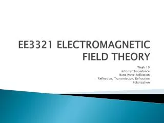
FD Solution of the 1-D Wave Equation / FD-Lösung der 1D Wellengleichung Normalized 1-D FD wave equation / Normierte 1D FD Wellengleichung Initial condition / Anfangsbedingung (Causality / Kausalität) Boundary condition / Randbedingung Discrete hyperbolic initial-boundary-value problem / Diskretes hyperbolisches Anfangs-Randwert-Problem
FD Method – 1-D FD Wave Equation – Flow Chart / FD-Methode – 1D FD-Wellengleichung - Flussdiagramm Start For all nx: 1-D FD wave equation / 1D FD Wellengleichung For all nx : Excitation / Anregung No Yes Stop
FD Method – 1-D Wave Equation – Example / FD-Methode – 1D Wellengleichung – Beispiel Raised cosine pulse with n cycles / Aufsteigender Kosinus-Impuls mit n Zyklen Raised cosine pulse with 2cycles / Aufsteigender Kosinus-Impuls mit 2 Zyklen Frequency / Frequenz Circular Frequency / Kreisfrequenz Time / Zeit t
FD Method – 1-D Wave Equation – Example / FD-Methode – 1D Wellengleichung – Beispiel Electric current density excitation: broadband pulse / Elektrische Stromdichteanregegung: breitbandiger Impuls Snapshots / Schnappschüsse Source point / Quellpunkt
Numerical Results – Validation / Numerische Ergebnisse – Validierung Numerical Results / Numerische Ergebnisse Validation / Validierung Compare numerical results with analytical solutions or with other numerical solutions. / Vergleiche die numerischen Ergebnisse mit analytischen Lösungen oder anderen numerischen Lösungen
Numerical Results – Validation / Numerische Ergebnisse – Validierung • Plane Wave Solution of the Homogeneous Case – • No sources, no boundaries! / • Ebene Wellen als Lösung des homogenen Falles – • Keine Quellen, keine Ränder! • Gives the correct characteristic, but not the correct amplitude and • no reflections at the boundaries! / • Gibt die korrekte Charakteristik, aber nicht die korrekte Amplitude und keine Reflexionen an den Rändern wieder! • 2. Green’s Function Solution of the Inhomogeneous Case – • “Point” source, but no boundaries, • if we use the free-space Green’s function! / • Lösung über Greensche Funktion für den inhomogenen Fall –„Punkt“quelle, aber keine Ränder, wenn wir die • Greensche Funktion für den Freiraum verwenden! • Gives the correct characteristic and correct amplitude, but no reflections • at the boundaries! / • Gibt die korrekte Charakteristik und die korrekte Amplitude, aber keine Reflexionen an den Rändern wieder!
FD Method – 1-D Wave Equation – Example / FD-Methode – 1D Wellengleichung – Beispiel Homogeneous scalar 1-D wave equation for the electric field strength / Homogene, skalare 1D-Wellengleichung für die elektrische Feldstärke Splitting of the 1D wave operator / Aufspaltung des 1D-Wellenoperators Hyperbolic partial differential equation / Hperbolische partielle Differentialgleichung One-way wave equation / “One-way” Wellengleichung
FD Method – 1-D Wave Equation – Example / FD-Methode – 1D Wellengleichung – Beispiel
FD Method – 1-D Wave Equation – Example / FD-Methode – 1D Wellengleichung – Beispiel Homogeneous scalar 1-D wave equation for the electric field strength / Homogene, skalare 1D-Wellengleichung für die elektrische Feldstärke Solution is a left and right propagating plane wave / Lösung ist eine nach links und rechts laufende ebene Welle A wave, which propagates for increasing time t in negative z direction / Eine Welle, die sich für zunehmende Zeit t in negative z-Richtung ausbreitet A wave, which propagates for increasing time t in positive z direction / Eine Welle, die sich für zunehmende Zeit t in positive z-Richtung ausbreitet
FD Method – 1-D Wave Equation – Example / FD-Methode – 1D Wellengleichung – Beispiel Consider an asymmetric triangular pulse / Betrachte einen asymmetrischen Dreiecksimpuls Excitation function / Anregungsfunktion Snapshots / Schnappschüsse This means, that the solution for all z and t is given by / Dies bedeutet, dass die Lösung für alle z und t gegeben ist durch Source point / Quellpunkt
FD Method – 1-D Wave Equation – Example / FD-Methode – 1D Wellengleichung – Beispiel Snapshots / Schnappschüsse Source point / Quellpunkt
FD Method – 1-D Wave Equation – Example / FD-Methode – 1D Wellengleichung – Beispiel ?
FD Method – 1-D Helmholtz Equation (Reduced Wave Equation)FD-Methode – 1D Helmholtz-Gleichung (Schwingungsgleichung) Homogeneous scalar 1-D wave equation / Homogene, skalare 1D-Wellengleichung 1-D Fourier transform with regard to time t / 1D Fourier-Transformation bezüglich der Zeit t 1-D inverseFourier transform with regard to circular frequency ω / 1D inverse Fourier-Transformation bezüglich der Kreisfrequenz ω
FD Method – 1-D Helmholtz Equation (Reduced Wave Equation)FD-Methode – 1D Helmholtz-Gleichung (Schwingungsgleichung) Homogeneous scalar 1-D wave equation / Homogene, skalare 1D-Wellengleichung Solution in the time domain / Lösung im Zeitbereich Homogeneous scalar 1-D Helmholtz wave equation (reduced wave equation) / Homogene, skalare 1D Helmholtz-Gleichung (Schwingungsgleichung) Solution in the frequency domain / Lösung im Frequenzbereich
FD Method – 1-D Helmholtz Equation (Reduced Wave Equation)FD-Methode – 1D Helmholtz-Gleichung (Schwingungsgleichung) Maxwell’s equations in the time domain / Maxwellsche Gleichungen im Zeitbereich Maxwell’s equations in the frequency domain / Maxwellsche Gleichungen im Frequenzbereich Electric field strength: plane wave / Elektrische Feldstärke: ebene Welle Magnetic field strength: plane wave / Magnetische Feldstärke: ebene Welle
FD Method – 1-D Helmholtz Equation (Reduced Wave Equation) FD-Methode – 1D Helmholtz-Gleichung (Schwingungsgleichung) Homogeneous scalar 1-D wave equation in the time domain / Homogene, skalare 1D-Wellengleichung im Zeitbereich Solution of the 1-D wave equation in the time domain / Lösung der homogenen 1D-Wellengleichung im Zeitbereich Solution of the 1-D Helmholtz equation in the frequency domain / Lösung der homogenen 1D-Helmholtz-Gleichung im Frequenzbereich Homogeneous, scalar 1-D Helmholtz equation in the frequency domain / Homogene, skalare 1D-Helmholtz-Gleichung im Frequenzbereich Solution of the 1-D wave equation for the magnetic field strength in terms of the electric field strength / Lösung der homogenen 1D-Wellengleichung für die magnetische Feldstärke als Funktion der elektrischen Feldstärke
FD Method – 1-D Wave Equation – Example / FD-Methode – 1D Wellengleichung – Beispiel Homogeneous scalar 1-D wave equations / Homogene, skalare 1D-Wellengleichungen Solutions / Lösungen Poynting vector / Poynting-Vector Poynting vector of the two plane waves / Poynting-Vektor der beiden ebenen Wellen
FD Method – 1-D Wave Equation – Example / FD-Methode – 1D Wellengleichung – Beispiel The plane wave solution gives the correct characteristic of the wave field, but the amplitude is not correct! This means we can not varify the numerical results with the plane wave solution of the homogeneous wave equation, because the simulated problem correspond to the solution of the inhomogeneous wave equation. / Die Ebene-Wellen-Lösung gibt die korrekte Charakteristik des Wellenfeldes wieder, aber die Amplitude der Wellenanteile ist nicht korrekt! Dies bedeutet, dass man die numerischen Resultate mit der Ebenen-Wellen-Lösung nicht vollständig verifizeiren kann, da die simulierte Situation mit der Lösung der inhomogenen Wellengleichung korrespondiert.
Electromagnetic Field of a “Point Source” Excitation in 1-D / Elektromagnetisches Feld einer „Punktquellen“anregung in 1D We consider a homogeneous infinite 1-D region / Wir betrachten ein homogenes, unendliches 1D-Gebiet Source point / Quellpunkt where we prescribe an electric current density Jex(z,ω) with the unit A/m2 at z=z0. / wobei wir eine elektrische Stromdichte mit der Einheit A/m2 an der Stelle z=z0vorgeben. Then, the unknown electric field strength is a solution of the inhomogeneous Helmholtz equation / Die unbekannte elektrische Feldstärke ist dann Lösung der inhomogenen Helmholtz-Gleichung A solution for the electric field strength is given by the domain integral representation / Eine Lösung für die elektrische Feldstärke ist dann gegeben über die (Gebiets-) Integraldarstellung Convolution integral / Faltungsintegral 1-D scalar Green’s function / 1D skalare Greensche Funktion
Electromagnetic Field of a Point Source Excitation in 1-D / Elektromagnetisches Feld einer Punktquellenanregung in 1D Integral representation / Integraldarstellung 1-D scalar Green’s function in the frequency domain / 1D skalare Greensche Funktion im Frequenzbereich 1-D scalar Green’s function in the time domain / 1D skalare Greensche Funktion im Zeitbereich Unit step function / Einheitssprungfunktion Electric surface current density / Elektrische Flächenstromdichte Electric current density / Elektrische Stromdichte Property of the delta-distribution / Eigenschaft der Delta-Distribution
EM Field of a Point Source Excitation in 1-D / EM-Feld einer Punktquellenanregung in 1D The asterisk “*t “denotes convolution in time / Der Stern “*t “ bezeichnet eine Faltung in der Zeit
EM Field of a Point Source Excitation in 1-D / EM-Feld einer Punktquellenanregung in 1D Wave impedance of free space (vacuum) / Wellenwiderstand des Freiraumes (Vakuum) Solution for the x component of the electric field strength / Lösung für die x-Komponente der elektrischen Feldstärke
EM Field of a Point Source Excitation in 1-D / EM-Feld einer Punktquellenanregung in 1D
EM Field of a Point Source Excitation in 1-D / EM-Feld einer Punktquellenanregung in 1D Solution for the y component of the magnetic field strength / Lösung für die y-Komponente der magnetische Feldstärke Solution for the x component of the electric field strength / Lösung für die x-Komponente der elektrischen Feldstärke Solution for the z component of the Poynting vector / Lösung für die z-Komponente des Poynting-Vektors
EM Field of a Point Source Excitation in 1-D / EM-Feld einer Punktquellenanregung in 1D Normalization of the field components / Normierung der Feldkomponenten Normalized EM field components / Normierte EM-Feldkomponenten EM Field components / EM-Feldkomponenten
FD Method – 1-D Wave Equation – Example / FD-Methode – 1D Wellengleichung – Beispiel The Green’s function method gives the solution of the 1-D simulation area excited by a “point” source, which is in 1-D a singular electric surface current source. The singular source is independent of x and y. The reference solution gives the correct characteristic and correct amplitudes. But the solution doesn’t account for the reflections at the boundaries, because we used the free-space Green’s function. / Die Methode der Greenschen Funktion ermöglicht die Lösung des vorliegenden Problems, der Anregung des 1D-Simulationsgebietes durch eine „Punkt“quelle, die genauer gesagt in 1D eine singuläre elektrische Flächenstromdichte ist. Da die singuläre Quelle von x und y unabhängig ist. Die Charakteristik und Amplitude stimmt überein, nur die Reflexionen an den Rändern fehlen, was an der Verwendung der Greenschen Funktion für den Freiraum liegt.
FD Method – Properties / FD-Methode - Eigenschaften • Spatial and Temporal Discretization / • Räumliche und zeitliche Diskretisierung • Consistency / • Konsistenz • Dissipation / • Dissipation • Stability Condition / • Stabilitätsbedingung • Convergence / • Konvergenz
Derivation of the Numerical Dispersion Relation for the 1-D FD Scheme of 2nd Order / Ableitung der numerischen Dispersionsrelation für das 1D-FD-Schema 2ter Ordnung Stability by the von Neumann’s method (Fourier series method): Insert a complex monofrequent (monochromatic) plane wave into the discrete FD equations and analyze the spectral radius of the amplification matrix, where the spectral radius must be smaller equal one. Stabilität durch die von Neumannsche Methode (Fourier-Reihen-Methode): Setze eine komplex monofrequente (monochromatische) ebene Welle in die diskreten FD-Gleichungen ein und analysiere den spektralen Radius der Verstärkungsmatrix, wobei der spektrale Radius kleinergleich Eins sein muss. Complex monofrequent (monochromatic) plane wave / Komplex monofrequente (monochromatische) ebene Welle
Derivation of the Stability Condition for the 1-D FD Scheme of 2nd Order / Ableitung der Stabilitätsbedingung für das 1D-FD-Schema 2ter Ordnung Monofrequent (monochromatic) plane wave in the time domain / Monofrequente (monochromatische) ebene Welle im Zeitbereich Plane of constant phase / Ebene konstanter Phase
Derivation of the Stability Condition for the 1-D FD Scheme of 2nd Order / Ableitung der Stabilitätsbedingung für das 1D-FD-Schema 2ter Ordnung Insert discrete plane wave / Setze die diskrete ebene Welle into the FD scheme / in das FD-Schema ein with / mit it follows / folgt
Derivation of the Stability Condition for the 1-D FD Scheme of 2nd Order / Ableitung der Stabilitätsbedingung für das 1D-FD-Schema 2ter Ordnung
Derivation of the Stability Condition for the 1-D FD Scheme of 2nd Order / Ableitung der Stabilitätsbedingung für das 1D-FD-Schema 2ter Ordnung Define / Definiere which yields for the above equation / womit wir für die obere Gleichung erhalten
Derivation of the Stability Condition for the 1-D FD Scheme of 2nd Order / Ableitung der Stabilitätsbedingung für das 1D-FD-Schema 2ter Ordnung Define a new algebraic vector / Definiere einen neuen algebraischen Vektor Characteristic polynomial / Charakteristisches Polynom
Derivation of the Stability Condition for the 1-D FD Scheme of 2nd Order / Ableitung der Stabilitätsbedingung für das 1D-FD-Schema 2ter Ordnung Eigenvalues of the amplification matrix / Eigenwerte der Verstärkungsmatrix
Derivation of the Stability Condition for the 1-D FD Scheme of 2nd Order / Ableitung der Stabilitätsbedingung für das 1D-FD-Schema 2ter Ordnung Spectral radius / Spektraler Radius Unit circle / Einheitskreis This means for, that all eigenvalues a2 ≤ 1 are on the unit circle in the complex plane. / Dies bedeutet, dass alle Eigenwerte für a2 ≤ 1 auf dem Einheitskreis in der komplexen Ebene liegen.
Derivation of the Stability Condition for the 1-D FD Scheme of 2nd Order / Ableitung der Stabilitätsbedingung für das 1D-FD-Schema 2ter Ordnung
Derivation of the Stability Condition for the 1-D FD Scheme of 2nd Order / Ableitung der Stabilitätsbedingung für das 1D-FD-Schema 2ter Ordnung 1-D Stability Condition for an FD algorithm of 2nd order in space and time– CFL-Condition / 1D-Stabilitätsbedingung für einen FD-Algorithmus zweiter Ordnung in Raum und Zeit– CFL-Bedingung 2-D and 3-D Stability Condition for an FD algorithm of 2nd order in space and time– CFL-Condition / 2D- und 3D- Stabilitätsbedingung für einen FD-Algorithmus zweiter Ordnung in Raum und Zeit– CFL-Bedingung
Derivation of the Stability Condition for the 1-D FD Scheme of 2nd Order / Ableitung der Stabilitätsbedingung für das 1D-FD-Schema 2ter Ordnung Spectral radius / Spektraler Radius Spectral radius / Spektraler Radius
Derivation of the Stability Condition for the 1-D FD Scheme of 2nd Order / Ableitung der Stabilitätsbedingung für das 1D-FD-Schema 2ter Ordnung Spectral radius / Spektraler Radius Eigenvalues / Eigenwerte