Download
1 / 63
630 likes | 784 Vues
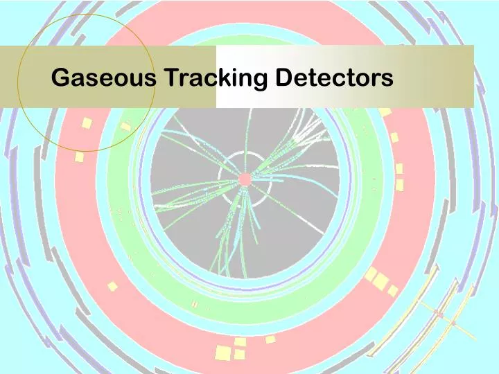
Gaseous Tracking Detectors. TexPoint fonts used in EMF. Read the TexPoint manual before you delete this box.: A A A A A A A A A. P 2. Overview. Straw trackers MWPCs TPCs Micropattern gas detectors Momentum measurement Thanks to Christian Joram and others from whom I borrowed slides.

E N D
Gaseous Tracking Detectors TexPoint fonts used in EMF. Read the TexPoint manual before you delete this box.: AAAAAAAAA
P 2 Overview • Straw trackers • MWPCs • TPCs • Micropattern gas detectors • Momentum measurement • Thanks to Christian Joram and others • from whom I borrowed slides Peter Hansen, Lecture on tracking detectors
P 3 Gaseous tracking detectors • Provides economic tracking over large areas • Measures primary ionization of charged tracks in the gas • Works by having avalances of secondary ionization • initiated when the primary ionization hits a small-area • anode. This provides built-in amplification. Peter Hansen, Lecture on tracking detectors
P 4 Signal formation Peter Hansen, Lecture on tracking detectors
P 5 An example gaseous tracker • The ATLASTransition Radiation Tracker • Installation • Design details • Simulation and performance • Calibration and Alignment • Particle ID
P 6 Transition Radiation Tracker Barrel • Straw diameter - 4 mm • Wire diameter - 30 μm • Polypropylene foil/fibre radiators End-caps • Gas 70%Xe+27%CO2+3%O2 • Xe for good TR absorption • CO2 > 6% for maximum operation stability • Gas gain 2.5104 Length: Total 6802 cm Barrel 148 cm End-cap 257 cm Outer diameter 206 cm Inner diameter 96-128 cm # straws: Total 372 832 Barrel 52 544 End-cap 319 488 # electronic channels 424 576 Weight ~1500 kg Peter Hansen, Lecture on gaseous tracking detectors
CMS ATLAS Atlas P 7 protons protons Peter Hansen, Rome seminar, 04-May-07
P 8 TRT performance 20 GeV beam ~1 TR hit ~7 TR hits 90%electron efficiency 10-2pion rejection Bd0J/ψ Ks0 High-γ charged particles (e.g. electrons) emit transition radiation (X-rays) when they traverse the radiators, detected in the straw tubes as larger energy deposition (8-10 KeV) TR threshold – electron/pion separation 6 keV 0.3 keV MIP threshold – precise tracking/drift time determination Peter Hansen, Lecture on geseous tracking detectors
P 9 The TRT Straw Peter Hansen, Lecture on gaseous tracking detectors
P 10 TRT commisioning 2008-2009 • The TRT barrel and end-caps were installed in their final position inside the cryostat in 2008 with all services. • One “splash-event” in 2008 was very useful for timing all the channels relative to each other. • Commissioning in 2009 with cosmic rays. The tracking resolution was found to be 160 microns. The High Threshold probability was found as expected.
The first collisions Dec2009 Peter Hansen, Lecture on gaseous tracking detectors
Gas Z A Emin Wi dE/dx Np Xe 54 131.3 5.49 10-3 g/cm3 8.4 eV 22 eV 1.23 MeV/(g/cm2) 44 ion/cm Co2 22 44 1.86 5.2 33 1.62 34 P 12 The TRT gas • 70% Xe (high amplification A=25000, absorbs X-rays) • 27% CO2(quenches ultraviolet, does not polymerize) • 3% O2(intercepts unwanted electrons) Peter Hansen, Lecture on tracking detectors
P 13 Drift of electrons in a B field New gas stabilizes drift velocity in B field. -and it does not eat glass Peter Hansen, Rome seminar, 04-May-07
P 14 GEANT4 Simulation Primary clusters formed according to PAI model Custom TR physics process Fiber radiator Photon x-sect Peter Hansen, Rome seminar, 04-May-07
P 15 Digitization simulation • Digitization includes • Diffusion and capture • Avalance formation • Electronics shaping • Noise • Reflections from ends • Propagation along wire • TOF and T0 fluctuation • Threshold fluctuations Peter Hansen, Rome seminar, 04-May-07
P 16 Custom ASIC readout Peter Hansen, Rome seminar, 04-May-07
P 17 The electric field • According to Gauss, the capacity per unit length, C, and the anode voltage, V0, determines the electric field: Integrating from the straw wall to the wire radius and equating The result toV0, gives Peter Hansen, Lecture on tracking detectors
P 18 Avalance development • The movement of a charge, Q, in a system with capacitance per unit length, C, by a distance dr gives a voltage signal v • Almost all avalance electrons are created in the last mean free path Peter Hansen, Lecture on tracking detectors
P 19 Shaping The positive ions drift to the cathode gives rise to: This contribution is about 50 times larger than that of the electrons. But it is a slow signal. By terminating the wire in a resistance, the signal is differentiated with a time constant, RC. For the TRT, the rise-time is 8ns and the duration only 20ns. Peter Hansen, Lecture on tracking detectors
P 20 Pulse shaping Problem: Long tail (much longer than the 25ns bunch spacing) from the positive ions moving outwards Solution: The ASDBLR front-end chip restores the baseline within ~20ns Peter Hansen, Rome seminar, 04-May-07
P 21 A simple calculation of A • Balancing concerns, the optimum gas amplification is 25000 • In any cascade process, we have • Leading to a total amplification of • At ionization energy, W=22eV, Xe presents a cross-section of • 2 10-16 cm2and the electron has a mean free path of Peter Hansen, Rome seminar, 04-May-07
P 22 A simple calculation of A • The distance from the wire, where the avalance starts, is given by: • The Townsend coefficient is assumed to be proportional to the kinetic energy of the electrons • Assuming =log 2 / at threshold, we have Peter Hansen, Rome seminar, 04-May-07
P 23 A simple calculation of A • Finally we get • This leads for the TRT to the target amplification of 25000 at a voltage of 1513 Volts, probably by luck this is close to the true value 1530 Volts. Peter Hansen, Rome seminar, 04-May-07
P 24 Drift Chambers Peter Hansen, Lecture on tracking detectors
P 25 The driftvelocity - naively • Assuming the electron is brought to halt at each collision and that the mean free path is independent of energy, we have at 1mm from a TRT wire: • The correct answer is Peter Hansen, Lecture on tracking detectors
P 26 Complications • The difference between prediction and fact is due to: • Dependence on electron energy of cross-section • (mainly the Ramsauer minimum around 1eV) • The quencher gas. • The magnetic field bending the drift-trajectories up/down • Diffusion Peter Hansen, Lecture on tracking detectors
P 27 modifications from quencher gas Peter Hansen, Lecture on tracking detectors
P 28 Diffusion (no field case) • The mean velocity of a particle in an ideal gas is given by Maxwell: • According to kinetic theory, a collection of particles localized at x=0 at t=0, will later have a distribution: • Where D is the diffusion coefficient Peter Hansen, Lecture on tracking detectors
P 29 The diffusion coefficient • According to statistical mechanics: • where the mean free path for an ideal gas is: • By substitition: Peter Hansen, Lecture on gaseous tracking detectors
P 30 Diffusion in an electric field • A classical argument by Einstein gives for an ideal gas in thermal equilibrium with the drifting ions: • In practice, we parametrize the spread of the coordinate in • the drift direction as: • Where the characteristic energy • can be calculated for known cross-sections and energy-losses • of the electron-gas collisions. Peter Hansen, Lecture on gaseous tracking detectors
P 31 The TRT resolution • The gasses in the TRT have a characteristic energy of about 2 eV. Thus we have for the coordinate perpendicular to the wires a spread of 0.114mm: • For an average of 10 primary ion pairs, the distance of the closest electron to the wire has a spread of about 0.012mm • The drift-time binning in 3.125ns contributes 0.043mm • Noise and gain variations gives 0.035mm • Uncertainties in wire position and time=0 gives 0.036mm • All together this gives a coordinate resolution of about 0.132mm, in excellent agreement with detailled calculations – and with data. Peter Hansen, Lecture on gaseous tracking detectors
P 32 Drift time simulation • The leading edge of signal gives the drift time of the ionization electrons and hereby the distance from the charged particle to the wire • The simulation includes diffusion, Lorentz-forces, signal propagation and shaping, channel-to-channel fluctuations in threshold and noise amplitudes (deduced from the observed noise levels), the time structure of noise – and more Peter Hansen lecture on gaseous tracking detectors
P 33 CTB data and simulation 100 GeV pions Residuals fromThomas Kittelmann thesis Sigma=0.132mm Perfect agreement! But only if using an average threshold of 161eV - where previous it was 300eV. The explanation is probably new noise and threshold fluctuations in MC – but there is no profound understanding. Peter Hansen lecture on gaseous trackling detectors
P 34 CTB data and simulation • Also the Time Over Threshold is reasonably well simulated And the hit efficiency is predicted to 95% in agreement with data Peter Hansen, lecture on gaseous tracking detectors
P 35 Tracking performance in ATLAS Peter Hansen, Rome seminar, 04-May-07
P 36 Calibration • Calibration is concerned with T0, the R(t-T0) relation, the high threshold probability and noise removal. • The ”V-plot” of time versus track impact position is used Peter Hansen, Rome seminar, 04-May-07
P 37 Calibration • The tip of the V yields T0 (and, if a single wire is plotted, • also the wire position). • The peak position in each 3ns bin of t-T0 yields R(t-T0) • (Note that the average position is not good because of tails at long arrival times for tracks passing close to the wire) Peter Hansen, Rome seminar, 04-May-07
Electron Identification in test beam P 38 Performace of combined pion rejection at 90% electron efficiency Universality of the HT probability Peter Hansen, Rome seminar, 04-May-07
P 39 Multiwire proportional counters • In 1968 it was shown by Charpak that an array of many closely spaced anode-wires in the same chamber could each act as an independent proportional counter. • This provided an affordable way of measuring particles over large areas, and the technique was quickly adopted in high energy physics. • Later it has found applications in all kinds of imaging of X-rays or particles from radioactive decay. Peter Hansen, Lecture on tracking detectors
P 40 Multiwire proportional counters Peter Hansen, Lecture on tracking detectors
P 41 Second coordinate –some ideas Peter Hansen, Lecture on tracking detectors
P 42 The TPC Peter Hansen, Lecture on tracking detectors
P 43 The TPC end-plate Peter Hansen, Lecture on tracking detectors
P 44 The TPC field cage • Experience shows that the greatest challenge in a TPC is to maintain a constant axial electric field. • This field is made by electrodes on the inner and outer cylinders • of the Field Cage, connected to a resistor chain. • Some useful elements are: • A Gating Grid to avoid space-charges. • Tight mechanical tolerances wrt the ideal cylindrical shape (while keeping the material budget low). • Severe cleaniness, (the tiniest piece of fiber in the cage may short-cut two electrodes and distort the field.) • As little as possible of insulator exposed to the drift-volume to avoid build-up of charge on the insulator. • Perfect matching of equipotential surfaces at the end plane is needed to avoid transverse field components. Peter Hansen, Lecture on tracking detectors
P 45 Electron drift in E and B fields • The TPC is immersed in a magnetic field parallel to the electric field. • this Langevin equation becomes in the stationary state • Introducing the mobility • and the cyclotron frequency • we get Peter Hansen, Lecture on tracking detectors
P 46 Electron drift in E and B fields • Solving for the drift velocity: • Since the coordinate resolution is high in the azimuthal direction, in order to measure the momentum well, a component of the velocity due to field distortions is very dangerous. But high helps! • At high , vD is suppressed by powers of • except for the effect of a B component. However, B is zero on the average according to Ampere. Peter Hansen, Lecture on tracking detectors
P 47 Electron diffusion in E and B fields • In the transverse projection an electron follows the arc of a circle with radius = vT /, where the mean squared velocity projected onto the transverse plane is: • After a time, t, the electron has reached a transverse distance of • so the spread after one collision is: Peter Hansen, Lecture on tracking detectors
P 48 Electron diffusion in E and B fields • After a longer time, the transverse spread is • Thus in large magnetic fields the transverse diffusion is reduced by a factor 1+22 • e.g. for Ar/Ethane and B=1.5Tesla the reduction is a factor 50. This is what makes a TPC possible! • Thus you can get a precision of about • for about 30 points on each track over a 1m-2m radial distance from the collision point. • Note that this is without any significant multiple scattering and with a good resolution also in the longitudinal direction. • It is also relatively CHEAP, since it is mainly gas. Peter Hansen, Lecture on tracking detectors
P 49 The ALEPH TPC Peter Hansen, Lecture on tracking detectors
P 50 TPC calibration Peter Hansen, Lecture on tracking detectors