Download
1 / 48
500 likes | 755 Vues
Shape Optimization for Elliptic Eigenvalue Problems. Chiu-Yen Kao Collaborators: He Lin, Yuan Lou, Stanley Osher, Fadil Santosa, Eli Yabolnovich, Eiji Yanagida IPAM, Numerics and Dynamics for Optimal Transport April 17, 2008. Control the resonance frequencies of devices:

E N D
Shape Optimization for Elliptic Eigenvalue Problems Chiu-Yen Kao Collaborators: He Lin, Yuan Lou, Stanley Osher, Fadil Santosa, Eli Yabolnovich, Eiji Yanagida IPAM, Numerics and Dynamics for Optimal Transport April 17, 2008
Control the resonance frequencies of devices: Maximize or minimize certain frequencies Maximize the gap between adjacent frequencies Maximize the ratio between real part and imaginary part of eigenvalues (quality factor optimization) Minimize the principle eigenvalue Application: Vibration system control Photonic crystal design Optical Resonator Population biology Motivation
Goal: Minimize a certain design objective such that is the eigenvalue of subjects to boundary condition on and is the elliptic differential operator. Shape Optimization for Elliptic Eigenvalue Problem
Motivation I : Shape of the drum Consider an open bounded , a positive , and satisfies the elliptic eigenvalue problem The eigenvalues are Q1:Shape problem: Q2:Composition problem:
Theoretical Results Q1:Shape problem: • Rayleigh (1877) conjectured, and Faber (1923) and Krahn (1925) proved, that if you fix the area of a drum, the lowest eigenvalue is minimized uniquely by the disk. • Payne, Pólya, and Weinberger conjecture (1955): The disk maximizes the ratio of to has been proved by Ashbaugh and Benguria (1992) Q2:composition problem: • Krein (1955) provided one dimensional optimal density distribution for maximal and minimal . • Cox and McLaughling (1993): minimal for higher dimensions.
Numerical Approach Q2:composition problem: Let Find shape optimization problem:
Shape Optimization of a drum head with a fixed domain Let be a domain inside , and Solve the optimization: Subject to the constraint: Eigenvalue Separation for Drums
The set is defined by The vector field is the displacement of . Shape Mapping
Framework of Murat-Simon: Let be a reference domain. Consider its variations with Definition: the shape derivative of at is the Frechet differential of at . Shape Derivative
Compute shape derivatives Shape Derivatives of Eigenvalues and Area
subject to use Lagrange multiplier method: the necessary condition for a minimizer is together with the constraint allows us, in principle, to find and . Lagrange Multiplier Method
Shape derivative Gradient descent algorithm for the shape The normal advection velocity of the shape is . We solve the level set equation: Because of , we need to have . Then . Gradient Ascent
Shape Optimization of a photonic crystal with a fixed domain Let be a domain inside , and We begin with a shape with and we want to maximize Motivation II : Photonic Crystal
Dielectric: 1 : 11.4 Initial Gap: none Final Gap: 0.1415 Maximize Band Gap
Dielectric: 1 : 11.4 Initial Gap: none Final Gap: 0.0989 Maximize Band Gap
Design the material to have lower loss of energy Mechanics Systems Ex: damped mass spring Electrical Systems Ex: RLC circuit, quartz crystal Optical Systems Ex: photonic crystal Pictures: http://en.wikipedia.org/wiki/Quartz_clock http://minty.stanford.edu/PBG/ Motivation III: Quality Factor Optimization
The Mass Spring System (1) The displacement satisfies: (1) For small damping , the solution is The total energy is and where the period .
The Mass Spring System (2) The quality factor is defined as :
1-D Schrödinger’s Equation • Finite potential well:
Optical Resonator • One-Dimensional Case • Higher-Dimensional Case • Goal: minimize the quality factor
1-D Forward Eigenvalue Solver (1) • Solve • by finite element method. Apply the test function • By incorporating the boundary condition
1-D Forward Eigenvalue Solver (2) Thus The equation can be written as It is a nonlinear Eigenvalue Problem !!
1-D Forward Eigenvalue Solver (3) • The equation can be written as
2-D Forward Eigenvalue Solver (1) • Boundary Integral Method • It is a nonlinear Eigenvalue Problem !!
2-D Forward Eigenvalue Solver (3) • Nonlinear Eigenvalue Problem: (Newton’s method) inverse iteration
Gradient Flow In terms of a single mode damped oscillator, the quality factor is proportional to the ratio between the real part and the imaginary part of the eigenvalue. Our goal here is to maximize the quality factor subject to the wave equation we discussed previously which can be written in the general eigenvalue problem Suppose there is a small perturbation s.t. We keep only the first order term Premultiplying by the corresponding eigenvector leads to Thus
Consider the elliptic eigenvalue problem with indefinite weight Let be a domain inside , and Solve the optimization: Subject to the constraint: IV: Eigenvalue with Indefinite Weight
where represents the density of a species and is the growth rate. 1. If , uniformly as 2. If , uniformly as The effect of dispersal and spatial heterogeneity in population dynamics. Diffusive Logistic Equation
Theorem: When is an interval, then there are exactly two global minimizers of . For the logistic model, this means that a single favorable region at one of the two ends of the whole habitat provides the best opportunity for the species to survive. Minimizers in 1D
In general domain: open question Suppose If then is not minimal. In particular, the strip at the end with much longer edge can’t be the optimal favorable region. Minimizers in High Dimensions
The End Thank you