Download
1 / 52
520 likes | 724 Vues
More Complex Graphics in R. FISH 397C Winter 2009 Evan Girvetz. © R Foundation, from http://www.r-project.org. Hands-on Exercise. Read in the possum.csv dataset to a data frame called possum Note that the first column of data should be the row names

E N D
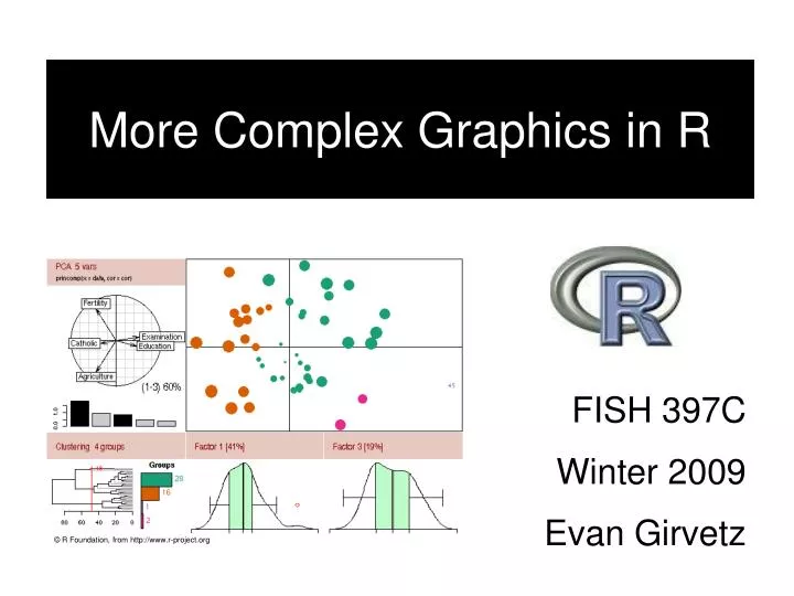
More Complex Graphics in R FISH 397C Winter 2009 Evan Girvetz © R Foundation, from http://www.r-project.org
Hands-on Exercise • Read in the possum.csv dataset to a data frame called possum • Note that the first column of data should be the row names • There are column headings for the other columns
possum Data Frame • Look at data frame > head(possum) case site Pop sex age hdlngthskullwtotlngthtaillfootlgthearconch eye chest belly C3 1 1 Vic m 8 94.1 60.4 89.0 36.0 74.5 54.5 15.2 28.0 36 C5 2 1 Vic f 6 92.5 57.6 91.5 36.5 72.5 51.2 16.0 28.5 33 C10 3 1 Vic f 6 94.0 60.0 95.5 39.0 75.4 51.9 15.5 30.0 34 C15 4 1 Vic f 6 93.2 57.1 92.0 38.0 76.1 52.2 15.2 28.0 34 C23 5 1 Vic f 2 91.5 56.3 85.5 36.0 71.0 53.2 15.1 28.5 33 C24 6 1 Vic f 1 93.1 54.8 90.5 35.5 73.2 53.6 14.2 30.0 32
Plotting Multiple Columns • Plot three columns at one time > possum[,c(6,8,9)] > plot(possum[,c(6,8,9)])
Multiple Graphs on One Layout • Look up mfrow and mfcol under par > ?par • mfrow: multiple plots on one graph filled by row • mfcol: same but by column
Multiple Graphs on One Layout The mfrow (or mfcol) command needs to be given to par prior to making the plots > par(mfrow=c(2,3)) Now draw plots in the order you want them displayed > plot(possum$hdlngth~possum$totlngth) > plot(possum$hdlngth~possum$taill) > plot(possum$totlngth~possum$taill) > hist(possum$hdlngth) > hist(possum$totlngth) > hist(possum$taill)
Hands-on Exercise • Create a plot with three graphs across • 1: head length vs. total length (x vs y) • 2: Histogram of total length • 3: Histogram of head length • Add more informative labels and titles • “Head Length” • “Tail Length” • “Total Length”
Making customized layouts layout(mat, widths = rep(1, ncol(mat)), heights = rep(1, nrow(mat)), respect = FALSE) mat a matrix object specifying the location of the next N figures on the output device. Each value in the matrix must be 0 or a positive integer. If N is the largest positive integer in the matrix, then the integers {1,...,N-1} must also appear at least once in the matrix. widths a vector of values for the widths of columns on the device. Relative widths are specified with numeric values. Absolute widths (in centimetres) are specified with the lcm() function (see examples). heights a vector of values for the heights of rows on the device. Relative and absolute heights can be specified, see widths above.
layout: custom layouts > mat <- matrix(c(1,1,3,2), 2, 2, byrow = TRUE) > mat > lay1 <- layout(mat=mat) > layout.show(lay1)
layout: custom layouts > mat <- matrix(c(1,1,0,2), 2, 2, byrow = TRUE) > lay1 <- layout(mat=mat) > layout.show(lay1)
layout: custom layouts > mat <- matrix(c(1,1,1,1,2,3), 3, 2, byrow = TRUE) > lay1 <- layout(mat=mat) > layout.show(lay1)
layout: custom layouts > plot(possum$hdlngth~possum$totlngth) > hist(possum$hdlngth) > hist(possum$totlngth)
layout: custom layouts > mat <- matrix(c(2,0,1,3),2,2,byrow=TRUE) > lay1 <- layout(mat, c(3,1), c(1,3), TRUE) > layout.show(lay1)
Simple Analyses: hist > ?hist # look at the help for hist > hdlngth.hist <- hist(possum$hdlngth) > totlngth.hist <- hist(possum$totlngth) > totLngth.hist ## look at totLngth.hist > plot(hdlngth.hist)
barplot > ?barplot > barplot(hdlngth.hist$counts) > par(mfrow= c(1,2)) > barplot(hdlngth.hist$counts) > barplot(hdlngth.hist$counts, horiz = T)
barplot > par(mfrow= c(1,2)) > barplot(hdlngth.hist$counts) > barplot(hdlngth.hist$counts, horiz = T)
Hands-on Exercise • Add these plots in this order • Scatter plot • totlngth histogram • hdlnth histogram
Changing the Margin Sizes > ?par # look at help for mar > par(mar = c(par(mar=c(3,3,1,1))) > par(mar = c(par(mar=c(0,3,1,1))) > par(mar = c(par(mar=c(3,0,1,1)))
Hands on Exercise Redo your layout using these margin sizes for the three plots in this order > par(mar = c(par(mar=c(3,3,1,1))) > par(mar = c(par(mar=c(0,3,1,1))) > par(mar = c(par(mar=c(3,0,1,1)))
Linear Regression : lm Use linear modeling: > totHd.lm <- lm(hdlngth ~ totlngth, data = possum) > summary(totHd.lm) > totHd.lm$coefficients > totHd.lm$residuals
Linear Regression : lm • Linear regression diagnostic graphs > plot(totHd.lm)
Adding lines to plots: abline > ?abline # look at the help for abline > par(mfrow = c(1,1)) > plot(possum$hdlngth~possum$totlngth) > abline(totHd.lm, lwd = 2, lty = 2)
Hands-on Exercise • Now add a trend line to the scatter plot in your layout
Text Expressions > coefA <- totHd.lm$coeficients[1,1] > coefB <-totHd.lm$coeficients[2,1] > text(x=80,y=101, expression(tailLen == 42.7 + 0.573 * (headLen) ))
Hands On Exercise • Add this equation to the scatter plot in your layout • Write the layout to a .png file and view in a graphics viewer
Lattice Graphics > library(lattice) > attach(possum) The lattice library must be loaded to use the lattice graphical functions
Lattice Graphics dotplot(factor ~ numeric,..) # 1-dim. Display stripplot(factor ~ numeric,..) # 1-dim. Display barchart(character ~ numeric,..) histogram( ~ numeric,..) densityplot( ~ numeric,..) # Density plot bwplot(factor ~ numeric,..) # Box and whisker plot qqmath(factor ~ numeric,..) # normal probability plots splom( ~ dataframe,..) # Scatterplot matrix parallel( ~ dataframe,..) # Parallel coordinate plots cloud(numeric ~ numeric * numeric, ...) # 3D surface wireframe(numeric ~ numeric * numeric, ...) # 3D scatterplot
Detach the possum data set > detach(possum)
Other Graphics and Expressions > symbols(0,0,circles=0.95,bg="gray", xlim=c(-1,2.25),ylim=c(1,1),inches=FALSE)
Other Graphics and Expressions > xVals <- c(1,3,4) > yVals <- c(4,2,3) > circleSizes <- c(.1, .2, .3) > symbols(xVals , yVals ,circles= circleSizes, bg="gray”, xlim = c(0,5), ylim = c(0,5),inches=FALSE)
Other Graphics and Expressions > symbols(xVals , yVals ,circles= circleSizes, bg=c(“red”, “green”, “blue”), xlim = c(0,5), ylim = c(0,5),inches=FALSE)
Other Graphics and Expressions > symbols(0,0,circles=0.95,bg="gray", xlim=c(-1,2.25),ylim=c(1,1),inches=FALSE) > text(1.75,0,expression("Area" ==pi*phantom("'") *italic(r)^2))
Other Graphics and Expressions > symbols(0,0,circles=0.95,bg="gray", xlim=c(-1,2.25),ylim=c(1,1),inches=FALSE) > text(1.75,0,expression("Area" ==pi*phantom("'") *italic(r)^2)) > arrows(0,0,-.95,0,length=.1,code=3)
Other Graphics and Expressions > symbols(0,0,circles=0.95,bg="gray", xlim=c(-1,2.25),ylim=c(1,1),inches=FALSE) > text(1.75,0,expression("Area" ==pi*phantom("'") *italic(r)^2)) > arrows(0,0,-.95,0,length=.1,code=3) > text(-0.45,-strheight("R"), expression(italic(r) == 0.95))
Finding Locations: locator() > location <- locator(n=1) Now click on the graphic where you’d like the label > text(location$x,location$y, expression("Area"==pi*phantom("'")*italic(r)^2))