WG 3: Overview status report

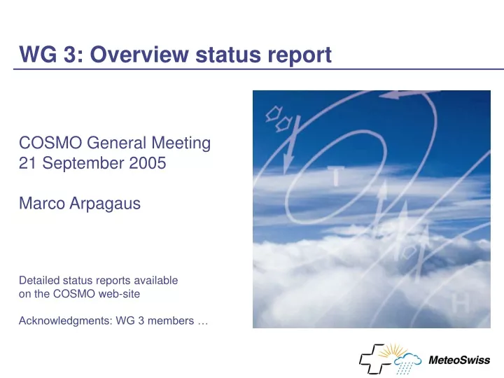
WG 3: Overview status report COSMO General Meeting 21 September 2005 Marco Arpagaus Detailed status reports available on the COSMO web-site Acknowledgments: WG 3 members …

WP 3.1: Planetary boundary layer • 3.1.1: Surface transfer scheme and turbulence scheme • 3.1.1.1 (top): Single column model, etc. • 3.1.1.2 (top): Reorganisation of the turbulence scheme • 3.1.1.3 (top): Extended documentation • 3.1.1.4: … • 3.1.1.5: … • 3.1.1.6 (top): Merge with 3-d approach • 3.1.2: Special boundary layer matters

The single column (SC) framework for LM - A testing tool : • SC-framework is a set of modules that can be added to a subset of existing LM-modules • The LM-modules are mainly those below ‘organise_physics.f90’ • The additional modules contain a complex data structure, which include pointers to the LM variable fields • The SC-framework enables the following functionality: • A SC-model run, using the LM-routinesfor physical calculations including the vertical flux divergence (slow_tendencies.f90) and using the INPUT-files for controlling the physics • The SC-run is hydrostatic with moving vertical -levels and geostrophic wind forcing • The model level configuration can be done by a configuration file specifying arbitrary pressure levels for the atmosphere and height levels of the soil. The configuration pressure levels define the corresponding -levels • Initial variable profiles and those for possible model forcing are extracted from a measurement file • The data in the measurement file include variable names and -units • Variable values of the measurement file are converted if possible to model variablesand model units by the help of a iterative variable- and unit conversion toolforcing by not-model-variables • Iterative calculation of pressure values if only height based measurements are present Zürich 2005 COSMO Matthias Raschendorfer

Variables that are chosen for forcing or needed for the initial state are vertically interpolated on model levels and stored in internal time series • The time series are interpolated by cubic splines on model time • Assimilation by either overwriting the model values by the values of the interpolated time series • or by combination with model values in order to minimise the resulting error • This includes an estimate of the interpolation error and the model time step error • and implicit error propagation for variable conversion and model calculations that are located within the framework • Chosen subroutines of LM may be shifted towards the framework with a modified declaration header to participate on the error propagation facilitysensitivity tests • Model forcing at different assimilation points regarding to the variable kind (prognostic, diagnostic, external, time tendency, etc.) • ASCII model output in the form of a measurement file for arbitrary forcing with model data • Output in structured ASCII files forvisualisation (at the moment by UNIRAS) • Diagnostic levels (0m, 2m, 10m, 850hPa, ...) are implicitly considered for input and output • Calculation of correction tendencies belonging to the forcing by the grid point output of a 3D LM run and forcing an other SC-run with those 3D correction tendencies (not yet ready) • Calculation of cost functions for predefined forcing variables (only in preparation) variational parameter optimisation • Current problem: The whole thing has to be carefully tested before safe use!! COSMO Zürich 2005 Matthias Raschendorfer

WP 3.1: Planetary boundary layer • 3.1.1: Surface transfer scheme and turbulence scheme • 3.1.1.1 (top): Single column model, etc. • 3.1.1.2 (top): Reorganisation of the turbulence scheme • 3.1.1.3 (top): Extended documentation • 3.1.1.4: … • 3.1.1.5: … • 3.1.1.6 (top): Merge with 3-d approach • 3.1.2: Special boundary layer matters

WP 3.2: Soil processes • 3.2.1: Multi-layer soil model • 3.2.1.1 (top): Operational implementation of the multi-layer soil model • 3.2.1.2: Usage of satellite derived (weekly updated) plant cover • 3.2.1.3 (top): Revision of external parameters for plants • 3.2.2: Implementation of lake model into the LM • 3.2.3: Intercomparison of soil models in the framework of soil moisture validation

WP 3.2.3 (Loglisci)

WP 3.3: Convection • 3.3.1 (top): Implementation and testing of alternative (deep) convection schemes • 3.3.2 (top): Shallow convection on the meso-g scale

WP 3.3.2 (Seifert)  poster LMK

WP 3.3.2 (Seifert)  poster

WP 3.4: Microphysics • 3.4.1: Three-category ice scheme

WP 3.5: Clouds • 3.5.1: Validation of boundary layer clouds • 3.5.2 (top): Testing sub-grid scale cloudiness approaches

WP 3.5.1 (Heise)  poster • There is a long lasting problem of LM to rapidly dissolve low level stratus or stratocumulus in late autumn and in winter. • According to earlier experiments by Dmitrii Mironov the problem might be fixed by setting back the minimum value of the vertical diffusion coefficient to zero. • This coefficient was introduced some years ago to avoid long lasting overcast situations over water areas. Following a reduction of evaporation over water in April 2004 this minimum vertical diffusion might turn up to be unnecessary. • The effect of a zero minimum vertical diffusion was tested in a parallel experiment for the period 1 October 2004 to 31 December 2004.

WP 3.5.1 (Heise)  poster • large improvements for cloud cover (good!) • negligible changes for 2m temperature and dew point (not so good!) • drastic degradation for (weak) precipitation and (turbulent) gusts (very bad!)

WP 3.5: Clouds • 3.5.1: Validation of boundary layer clouds • 3.5.2 (top): Testing sub-grid scale cloudiness approaches

WP 3.5.2 (Avgoustoglou)  poster Aim: • Validate (and tune) statistical cloud scheme, particularly the interaction with the radiation scheme. • Start with tuning the ‘cloud cover at saturation’ (zclc0) and the ‘critical value of the saturation deficit’ (zq_crit) parameters.

WP 3.5.2 (Avgoustoglou)  poster Conclusions: • The forecasted low cloud cover was sensitive to the parameters zq_crit and zclc0 of the statistical cloud scheme. • Vertical diffusion coefficients did not show any effect to this particular test case. • The results, although versatile, look realistic, leaving space for possible tuning. • Due to the more general impact the results might have to the physics of the model further understanding and testing must be considered before any operational implementation of the statistical cloud scheme.

WP 3.6: Radiation • 3.6.1: Cloud-radiation interaction • 3.6.2: Evaluate possible inclusion of 3-d effects in current scheme • Gridscale parameterization of topographic effects on radiation • Radiation calculation on a coarser grid – very first results with LMK

WP 3.6.1 (Bozzo et al.) Small discrepancies in clear sky profile are most probably due to out of date spectroscopic database used in GRAALS (= code used in LM) Water cloud parameterization used in GRAALS gain good results compared to “exact” multiple scattering computa-tions provided by RTX-3

WP 3.6: Radiation • 3.6.1: Cloud-radiation interaction • 3.6.2: Evaluate possible inclusion of 3-d effects in current scheme • Gridscale parameterization of topographic effects on radiation • Radiation calculation on a coarser grid – very first results with LMK

WP 3.6.2 (Buzzi et al.)  poster Surface temperature difference, 2004 12 11 12 UTC 2 km 7 km

WP 3.6.2 (Buzzi et al.)  poster Summary and conclusions • The Müller and Scherrer (2005) scheme for topographic effects on radiation has been implemented into the LM. • Some sensitivity case studies have been carried out. • The impact of the topographic effects (shadowing, slope angle, slope aspect, and sky view) is substantial at high resolution. • Some significant indirect impacts (feedbacks) related to snow melt, stability (turbulence), and low clouds, even at 7km. • Larger impact during the winter time due to sun elevation and snow conditions. • Surface thermal changes at high resolution have also secondary effects on thermal circulation.

WP 3.6.2 (Reinhardt) Aim: call radiation code more frequently  calculate radiation on a coarser grid LMK grid grid for radiation

WP 3.6.2 (Reinhardt) (Very) First results: • Overall: nearly neutral impact • Bottom and top radiative fluxes, averaged: neutral • Verification against 24-h precipitation sums: ok • Eye-inspection of visualized output: ok • Verification against SYNOP data: not yet done • Pointwise, of course, also bigger differences • Outlook: Systematic tests

WP 3.7: Sub-km version • 3.7.1: Use of LM to study intense convective precipitation events

WP 3.8: z-coordinate version • 3.8.1 (N.N.): Adaptation of the parameterization schemes

WP 3.9: Validation and related matters • 3.9.1: Testing the SC framework, running parameter tuning experiments, and validating (1-d) boundary layer processes • 3.9.2: Validation (3-d) of the boundary layer processes • 3.9.3 (top, N.N.): Development of a tool for extended parameter determination

WP 3.9.2 (Vogel et al.) • PBL too moist and too cold • Sensitivity experiments with different turbulence schemes however inconclusive, since ‘boundary conditions’ wrong: • too strong radiative forcing (due to wrong clouds) • too moist soil LM

WP 3.10: Tackle observed model deficiencies • 3.10.1: Cure overestimation of low precipitation in winter • 3.10.2: Improve diagnosis of convective and turbulent gusts • 3.10.3: Investigate reason for cold/moist bias in PBL • 3.10.4 (N.N.): Understand sharp increase in precipitation overestimation since November 2003

WP 3.10.2 (Heise)  poster Convective gusts, changes: • The effect of water loading is included in the buoyancy determination of downdrafts • The tuning parameter responsible for distributing the downward kinetic energy of the gusts to all horizontal directions is increased from sqrt(0.2) to sqrt(1/p). • If the convective precipitation rate is below 0.015 mm/h, convective gusts are suppressed. Improvements for test cases; verification results of test suite still pending.

WP 3.10.2 (Heise)  poster Turbulent gusts, changes: • Use Brasseur (2001) method • Add sqrt(TKE) of lowest layer Results of test suite are … … rather negative! Need to reformulate and try again …

Joint WG3-WG5 workshop (9.3.2005) Conditional verification (excerpt from the minutes): • WG3 provides a list of criteria to use for conditional verification. [done] • WG5 is invited to provide a tool (‘data finding tool’) that allows to easily and efficiently find days / grid-points which satisfy specific criteria. • WG5 is kindly asked to supply a conditional verification of the operational model suites on a regular basis. • Testing of the reference version should also include conditional verifications.

WG 3: Overview status report