Download
1 / 18
250 likes | 1.87k Vues
Materials for Lecture 08. Chapters 4 and 5 Chapter 16 Sections 3.2-3.7.3 Lecture 08 Bernoulli & Empirical.xls Lecture 08 Normality Test.xls Lecture 08 Parameter Est.xls Lecture 08 Normal.xls Lecture 08 Simulate a Reg Model.xls. Stochastic Simulation.

E N D
Materials for Lecture 08 • Chapters 4 and 5 • Chapter 16 Sections 3.2-3.7.3 • Lecture 08 Bernoulli & Empirical.xls • Lecture 08 Normality Test.xls • Lecture 08 Parameter Est.xls • Lecture 08 Normal.xls • Lecture 08 Simulate a Reg Model.xls
Stochastic Simulation • Purpose of simulation is to estimate the unknown probability distribution for a KOV so decision makers can make a better decision • Simulate because we can not observe and measure the KOV distribution directly • Want to test alternative values for control variables • Sample PDFs for random variables, calculate values of KOV for many iterations • Record KOV • Analyze KOV distribution
Stochastic Variables • Any variable the decision maker can not control is thought to be stochastic • In agriculture we think of yield as stochastic as it is subject to weather • For most businesses the prices of inputs and outputs are not directly controlled by management so they are stochastic. • Production may be random as well. • Include the most important stochastic variables in simulation models • Your model can not include all random variables
Stochastic Simulation • In economics we use simulation because we can not experiment on live subjects, a business or the economy without injury • In other fields they can fabricate an experiment • Health sciences they feed/treat multiple rats on different chemicals • Animal science feed multiple pens of steers, chickens, cows, etc. • Engineers run a motor under different controlled situations (temp, RPMs, lubricants, fuel mixes) • Vets treat different pens of animals with different meds • Agronomists set up randomized block treatments for a particular seed variety • All of these are just different iterations of “models”
Iterations, How Many are Enough? Specify the number of iterations in the Simetar simulation engine Specify the output variables’ names and location • Change the number of iterations based on nature of the problem -- 500 is adequate. • Some studies use 1,000’s because they are using a Monte Carlo sampling procedure which is less precise than Latin hypercube • Simetar uses a Latin hypercube so 500 is an adequate sample size
Normal Distribution • Normal distribution a continuous distribution that produces a bell shaped distribution with set probabilities • Parameters are • Mean • Standard Deviation • Normal distribution reaches to + and - infinity. • Can produce negative values so be careful • Can produce extremely high values • Most of us have memorized several probabilities for the normal distribution: • 66% of observation within +/- 1 of the mean • 95% of observation within +/- 2 of the mean • 50% of observations lie above and below the mean.
Simulating Random Variables • Normal distribution is used frequently, particularly when simulating a regression model • Parameters for a Normal distribution • Mean expressed as Ῡ or Ŷ • Standard Deviation σ (or SEP from a regression model) • Assume yield is a random variable and have production function data, such as: • Ỹ = a + b1Fert + b2 Water + ẽ • Deterministic component is: a + b1Fert + b2 Water • Stochastic component is: ẽ • Stochastic component, ẽ, is assumed to be distributed Normal • Mean of zero • Standard deviation of σe • See Lecture 8 Simulate a Reg Model.XLS
PDF and CDF for a Normal Dist. Probability Density Function Cumulative Distribution Function f(x) F(x) - + - +
Use the Normal Distribution When: • Use the Normal distribution if you have lots of observations and have tested for normality • Watch for infeasible values from a Normal distribution (negative yields and prices)
Problems with the Normal • It is easy to use, so it often used when it is not appropriate • It does not allow for extreme events (BS’s) • No way to account for record breaking outliers because the distribution is defined by Mean and Std Dev. • Std Dev is the “average” deviation from the mean and averages out BS’s • Market outliers are washed away in the average • It is the foundation for Sigma 6 • So it suffers from all of the problems of the Normal • Creates a false sense of security because it never sees a record braking outlier
Test for Normality • Simetar provides an easy to use procedure for testing Normality that includes: • S-W – Shapiro-Wilks • A-D – Anderson-Darling • CvM – Cramer-von Mises • K-S – Kolmogornov-Smiroff • Chi-Squared • Simetar’s Hypothesis Testing Icon (Ho Hi) provides a tab to “Test for Normality”
Simulating a Normal Distribution • Normal Distribution =NORM( Mean, Standard Deviation) =NORM( 10,3) =NORM( A1, A2) • Standard Normal Deviate (SND) =NORM(0,1) or =NORM() • SND is the Z-score for a standard normal distribution allowing you to simulate any Normal distribution • SND is used as follows: Ỹ = Mean + Standard Deviation*NORM(0,1) Ỹ = Mean + Standard Deviation*SND Ỹ = A1 + (A2 * A3) where a SND is in cell A3
Truncated Normal Distribution • General formula for the Truncated Normal =TNORM( Mean, Std Dev, [Min], [Max],[USD] ) • Truncated Downside only =TNORM( 10, 3, 5) • Truncated Upside only =TNORM( 10, 3, , 15) • Truncated Both ends =TNORM( 10, 3, 5, 15) • Truncated both ends with a USD in general form =TNORM( 10, 3, 5, 15, USD)
Example Model of Net Returns for a Business Model - Stochastic Variables -- Yield and Price - Management Variables -- Acreage and Costs (fixed and variable) - KOV -- Net Returns - Write out the equations and exogenous values Equations and their order
Program a Simulation Model in Excel/Simetar -- Input Data Section of the Worksheet A B C 1 VC / acre 150.0 2 VC / Y 0.25 3 Acre 100 10 4 Fixed Cost 5 Yield Mean & Std. Dev. 150 30 Price Mean & Std. Dev. 6 2 0.40 • See Lecture 08 Simulation Model with Simetar.XLS
Program Model in Excel/Simetar -- Generate Random Variables and Simulate NR A B C 13 Stochastic Yield Formulas in Column B 14 Mean 150 = B5 15 Std. Dev. 30 = C5 16 SND 0.362 = NORM ( ) 17 Random Yield 160.86 = B14 + B15 * B16 18 Stochastic Price 19 Mean 2.00 = B6 20 Std. Dev. 0.40 = C6 21 SND -0.216 = NORM ( ) 22 Random Price 1.9136 = B19 + B20 * B21 23 Receipts from Market 24 Yield 160.86 = B17 25 Price 1.9136 = B22 26 Acres 100 = B3 27 Receipts 30782.16 = B24 * B25 * B26 28 29 Calculate Costs 30 Fixed Cost 10 = B4 31 VC/acre 4000 = B1 * B3 32 VC/Y 2412.9 = B2 * B17 * B4 33 Total 6422.9 = Sum (B30 : B32) 34 Net Returns 24359.26 = B27 – B33 35
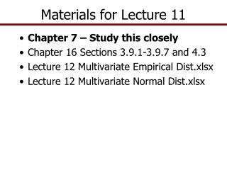
PDF for Bernoulli B(0.75) CDF for Bernoulli B(0.75) 1 .25 .25 .75 0 0 1 X 1 X PDF and CDF for a Bernoulli Distribution. Bernoulli Distribution • Parameter is ‘p’ or the probability that the variable is 1 or TRUE • Simulate Bernoulli in Simetar as • = Bernoulli(p) • = Bernoulli(0.25)
Bernoulli Distribution • Use Bernoulli in a conditional distribution as demonstrated: • It rains 20% of time during June and if it rains, the amount is distributed U(0.1, 0.9) Cell A2 =BERNOULLI(0.20) Cell A3 =UNIFORM(0.1, 0.9) * A2 • Probability of mechanical failure is 5%, cost of repair is $10,000, $20,000, or $30,000 Cell A4 =BERNOULLI(0.050) Cell A5 =DEMPIRICAL(10000, 20000, 30000) Cell A6 = A4 * A5