Download
1 / 18
190 likes | 391 Vues
Decision Tree Example. MSE 2400 EaLiCaRA Spring 2014 Dr . Tom Way. Decision Tree Learning (1).

E N D
Decision Tree Example MSE 2400 EaLiCaRA Spring 2014 Dr. Tom Way
Decision Tree Learning (1) • Decision tree induction is a simple but powerful learning paradigm. In this method a set of training examples is broken down into smaller and smaller subsets while at the same time an associated decision tree get incrementally developed. At the end of the learning process, a decision tree covering the training set is returned. • The decision tree can be thought of as a set sentences (in Disjunctive Normal Form) written propositional logic. MSE 2400 Evolution & Learning
Decision Tree Learning (2) • Some characteristics of problems that are well suited to Decision Tree Learning are: • Attribute-value paired elements • Discrete target function • Disjunctive descriptions (of target function) • Works well with missing or erroneous training data MSE 2400 Evolution & Learning
Decision Tree (goal?) (Outlook = Sunny Humidity = Normal) (Outlook = Overcast) (Outlook = Rain Wind = Weak) [See: Tom M. Mitchell, Machine Learning, McGraw-Hill, 1997] MSE 2400 Evolution & Learning
Day Outlook Temperature Humidity Wind PlayTennis D1 Sunny Hot High Weak No D2 Sunny Hot High Strong No D3 Overcast Hot High Weak Yes D4 Rain Mild High Weak Yes D5 Rain Cool Normal Weak Yes D6 Rain Cool Normal Strong No D7 Overcast Cool Normal Strong Yes D8 Sunny Mild High Weak No D9 Sunny Cool Normal Weak Yes D10 Rain Mild Normal Weak Yes D11 Sunny Mild Normal Strong Yes D12 Overcast Mild High Strong Yes D13 Overcast Hot Normal Weak Yes D14 Rain Mild High Strong No Play Tennis Data MSE 2400 Evolution & Learning
Building a Decision Tree • Building a Decision Tree • First test all attributes and select the one that would function as the best root; • Break-up the training set into subsets based on the branches of the root node; • Test the remaining attributes to see which ones fit best underneath the branches of the root node; • Continue this process for all other branches until • all examples of a subset are of one type • there are no examples left (return majority classification of the parent) • there are no more attributes left (default value should be majority classification) MSE 2400 Evolution & Learning
Finding Best Attribute • Determining which attribute is best (Entropy & Gain) • Entropy (E) is the minimum number of bits needed in order to classify an arbitrary example as yes or no • E(S) = ci=1 –pi log2 pi , • Where S is a set of training examples, • c is the number of classes, and • pi is the proportion of the training set that is of class i • For our entropy equation 0 log2 0 = 0 • The information gain G(S,A) where A is an attribute • G(S,A) E(S) - v in Values(A) (|Sv| / |S|) * E(Sv) MSE 2400 Evolution & Learning
Example (1) • Let’s Try an Example! • Let • E([X+,Y-]) represent that there are X positive training elements and Y negative elements. • Therefore the Entropy for the training data, E(S), can be represented as E([9+,5-]) because of the 14 training examples 9 of them are yes and 5 of them are no. MSE 2400 Evolution & Learning
Example (2) • Let’s start off by calculating the Entropy of the Training Set. • E(S) = E([9+,5-]) = (-9/14 log2 9/14) + (-5/14 log2 5/14) • = 0.94 MSE 2400 Evolution & Learning
Example (3) • Next we will need to calculate the information gain G(S,A) for each attribute A where A is taken from the set {Outlook, Temperature, Humidity, Wind}. MSE 2400 Evolution & Learning
Example (4) • The information gain for Outlook is: • G(S,Outlook) = E(S) – [5/14 * E(Outlook=sunny) + 4/14 * E(Outlook = overcast) + 5/14 * E(Outlook=rain)] • G(S,Outlook) = E([9+,5-]) – [5/14*E(2+,3-) + 4/14*E([4+,0-]) + 5/14*E([3+,2-])] • G(S,Outlook) = 0.94 – [5/14*0.971 + 4/14*0.0 + 5/14*0.971] • G(S,Outlook) = 0.246 MSE 2400 Evolution & Learning
Example (5) • G(S,Temperature) = 0.94 – [4/14*E(Temperature=hot) + 6/14*E(Temperature=mild) + 4/14*E(Temperature=cool)] • G(S,Temperature) = 0.94 – [4/14*E([2+,2-]) + 6/14*E([4+,2-]) + 4/14*E([3+,1-])] • G(S,Temperature) = 0.94 – [4/14 + 6/14*0.918 + 4/14*0.811] • G(S,Temperature) = 0.029 MSE 2400 Evolution & Learning
Example (6) • G(S,Humidity) = 0.94 – [7/14*E(Humidity=high) + 7/14*E(Humidity=normal)] • G(S,Humidity = 0.94 – [7/14*E([3+,4-]) + 7/14*E([6+,1-])] • G(S,Humidity = 0.94 – [7/14*0.985 + 7/14*0.592] • G(S,Humidity) = 0.1515 MSE 2400 Evolution & Learning
Example (7) • G(S,Wind) = 0.94 – [8/14*0.811 + 6/14*1.00] • G(S,Wind) = 0.048 MSE 2400 Evolution & Learning
Example (8) • Outlook is our winner! MSE 2400 Evolution & Learning
Next Level (1) • Now that we have discovered the root of our decision tree we must now recursively find the nodes that should go below Sunny, Overcast, and Rain. MSE 2400 Evolution & Learning
Next Level (2) • G(Outlook=Rain, Humidity) = 0.971 – [2/5*E(Outlook=Rain ^ Humidity=high) + 3/5*E(Outlook=Rain ^Humidity=normal] • G(Outlook=Rain, Humidity) = 0.02 • G(Outlook=Rain,Wind) = 0.971- [3/5*0 + 2/5*0] • G(Outlook=Rain,Wind) = 0.971 MSE 2400 Evolution & Learning
Next Level (3) • Now our decision tree looks like: MSE 2400 Evolution & Learning